


 Inglês (pdf)
 Artigo em XML
 Referências do artigo
 Enviar este artigo por email
 Citado por SciELO
  Similares em
SciELO
Similares em
SciELO 
 Permalink
1. INTRODUCTION
A prompt estimation of strong ground motion in the aftermath of a large earthquake is essential for early disaster response. One of the most popular services to provide strong motion parameters to all regions of the globe is ShakeMap, operated by the United States Geological Survey (USGS)1. There exist, however, systems dedicated exclusively to specific countries to achieve better spatial resolution and accuracy. For instance, a web-based quick estimation system of strong ground motion map for Japan is reported in2. For Istanbul Metropolitan area, ground motion parameter distribution maps are provided by the Istanbul Earthquake Rapid Response Network3. Strong motion parameters are recorded from in-place sensors, such as accelerometers. Other kind of in-place sensors are tide gauges, used to estimate tsunami inundation depths, and water depth sensors to monitor river overflow inundation. Recently, the integration of in-place sensors and remote sensors to identify damage in the infrastructure has been proposed. Tsunami inundation depth, fragility curves, and satellite radar images have been used to identify collapsed buildings4,5. Furthermore, collapsed buildings during the 2016 Kumamoto earthquake were identified using digital elevation models and strong motion parameters6.
Regarding strong motion parameters map in Peru, reports from Red Acelerográfica7, a strong motion network in the country, provides iso-acceleration map for each earthquake event. However, since the number of strong motion stations distributed in Peru is still low, the spatial resolution is coarse and there are only four levels of PGA. On the other hand, The Lima Metropolitan area does have a significant number of strong motion stations. Thus, strong motion parameters maps can be produced with better resolution. In this manuscript, we report the development of an interpolation system of strong motion parameters for Lima Metropolitan. The system is based on Kriging interpolation techniques and takes into account the soil amplification factors. The rest of the manuscript is structured as follows. The next chapter introduces the procedure and the components of the interpolation scheme. Section 3 reports an application of the system and an empirical evaluation on the 2021 Mw 6.0 Mala earthquake event. Section 4 provides some insights regarding the future work scheduled to improve the accuracy of the strong motion parameters map. Finally, our conclusions are drawn in the last section.
2. METHODOLOGY
2.1 INTERPOLATION METHOD
The Kriging interpolation approach is adopted to interpolate the parameters measured in the strong motion stations. In the Kriging approach, each strong motion station, located at coordinate xi, is modelled as a random variable, z(xi), with a certain expected value, E[Z(xi)], and a variance, Var(Z(xi)). Consider n measurements at xi∀i:1,…,n, we aim to estimate a value at x0, Z(x0). There are three main variations of the Kriging interpolation. When E[xi] is known and constant for all xi, then Z(x0) is estimated with the Simple Kriging approach:

where Z*(x0) denotes the estimation of Z(x0), wi denotes a weight factor for xi, and μ is the constant expected value for all Z(xi). When μ is unknown, Z(x0) is estimated with the Ordinary Kriging approach:

There is a third approach, referred as Universal kriging, that is used when E[xi] shows a trend, rather than being constant. Under this condition, Z*(x) is split into two terms

where μ(x) denotes the expected value as a function of the coordinate x, which contains a trend, and Y(x) denotes the random component with E[Y(x)]=0.
For the implementation of the strong motion parameter maps, the Ordinary Kriging approach is adopted. To compute the weight factors, the variance of the expected error,  , needs to be minimized. Thus, it is necessary to define in a closed form.
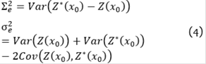
Then replacing Eq. (2) in Eq. (4) we obtain:

where Cij=Cov(Z(xi),Z(xj)) denotes the covariance between the Z(xi) and Z(xj). Then, the weight factors, wi, can be computed from the following optimization problem:

where C denotes the covariance matrix, c0 denotes a vector whose component i represents Ci0. Using the method of Lagrange multipliers, Eq. (6) is reduced to the following linear equation system:

where λ denotes the Lagrange multiplier. It is assumed that the covariance between two random variables, Cij, depends only on the distance between the stations, rather than their coordinates. That is, c(xi,xj)=c(h), where h denotes |xi-xj|. Furthermore, the covariance can be deduced from its relation with the semivariogram:

where the variogram function, γ(h), can be estimated from the semivariance:

2.2 SOIL AMPLIFICATION FACTORS
The soil amplification map provided in 8 is used in this study. The spatial resolution of the grid is about 250 m. The amplification factors are computed using the average transfer function method, which is computed from the transfer function between the ground surface and the engineering bedrock. In the manuscript, we define engineering bedrock as the layer associated with a shear-wave velocity value of 500m/s, in average. The shear wave velocity profiles, required to compute the transfer functions, were obtained from multichannel analysis of surface waves (MASW) measurements. The formula to estimate the amplification factor is

where AvTF denotes the average transfer function, f denotes the transfer function, and T denotes a period. In addition to Eq. 10, AvTF was estimated from its empirical relation with the time-averaged shear-wave velocity in the first ten meters and the soil dominant frequency. Researchers at CISMID are currently working to increase the extent of the soil amplification as more MASW measurements become available. Fig. 1a shows the current soil amplification map for Lima Metropolitan.

2.3 STRONG MOTION NETWORKS
Over the last years, different institutions have implemented strong motion networks in Peru. As a result, there is a significant number of acceleration sensors in Lima Metropolitan that has already recorded earthquakes of low/medium magnitude. The Geophysics Institute of Peru (IGP) manages the National Seismologic Center (CENSIS). According to 9, CENSIS has 169 strong motion stations spread countrywide, 59 of which are installed in Lima Metropolitan. The National Accelerometer’s Network of CISMID (REDACIS) has currently 39 stations distributed in Lima Metropolitan10. The Red Acelerográfica, administrated by the Graduate School of the Faculty of Civil Engineering, National University of Engineering, has 79 strong motion stations installed countrywide. The stations are installed in universities and departmental councils of the College of Engineers of Peru7.
2.4 PROCESSING CHAIN OF THE INTERPOLATION SYSTEM
Fig. 2 illustrates the processing chain of the interpolation system that is going to be followed in every earthquake event. The process requires two inputs: strong motion records and the soil amplification factor map. First, in the aftermath of an earthquake the strong motion records are collected and the parameters, such as the PGA and PGV, at the ground surface are computed. Then, using the amplification factors, the strong motion parameters at the engineering bedrock are estimated. Furthermore, the parameters are interpolated using the ordinary Kriging method. This stage implies (i) computing the semivariances (Eq. 9) from every pair of stations, (ii) fitting a semivariogram function, (iii) for each interpolation point, the covariance matrix (Eq. 8), the interpolation weights are computed (Eq. 7), and the interpolated values are computed (Eq. 2). Finally, the interpolated parameters map at the engineering bedrock is brought to the surface using the amplification factors.

3. EMPIRICAL EVALUATION
We evaluated the performance of the interpolation scheme on the Mw 6.0 Mala earthquake, occurred in June 22, 2021 at 21:54:17 (UTC-5). The epicenter was located 33 km southwest of the district of Mala, Lima, Peru. Fig. 1b depicts the 56 strong motion stations that recorded the event in Lima Metropolitan, five of which belong to Red Acelerográfica, 35 from REDACIS, and 16 from CENSIS. Fig. 3a shows the PGA estimated at the engineering bedrock. In Fig. 3b, the blue marks denote the semivariances, the red bars show the number of pair stations used to compute each semivariance, and the green line denotes the adjusted semivariogram. Fig. 4 shows the estimated PGA map at surface.

Fig. 3 (a) Estimated PGA at the engineering bedrock below the strong motion stations. (b) Fitting of the semivariogram.

The evaluation consists of removing one of the 56 records, hereafter referred to as test-PGA, and using the rest 55 records to compute the interpolation scheme. Then, the test record is compared with the interpolation-based PGA. The procedure was performed 56 times with a different record as test-PGA. Fig. 5a shows a comparison of the test-PGA with the recorded PGA. The average absolute value error is 31 gal, and the square root of the average of the squared error is 40.8 gal. Note that the error affects more at stations that recorded low PGA value, as observed in the ratio between the estimated and the recorded PGA (See Fig. 5c). Fig. 5b shows the absolute value errors at each station. It is observed that the most significant errors occurred under one of two conditions: (i) when the distance between the test station and its closest station is large. This error will be progressively reduced as more stations are planned to be installed in Lima Metropolitan; and (ii) when the test station is located within the boundary of the study area. Recall that the boundary is the limit between what can be considered an interpolation value and an extrapolation value. Thus, large errors at the boundary are somehow expected. Fig 5c suggests that there are overestimations at lower PGAs, while there are underestimations at large PGAs. Such an effect occurs when a test station represents a local minimum (maximum) and the nearby stations exhibit larger (lower) PGA.

4. FUTURE DEVELOPMENT
The current interpolation scheme uses the Ordinary Kriging method, which assumes a constant expected value. This is not precisely the case for earthquakes, as there is a trend in most ground motion models. It is already shown elsewhere that including the attenuation law improves the accuracy. However, to our knowledge, there is no attenuation law proposed for Peru. The attenuation trend will be fitted for each earthquake event to overcome this pitfall. For that purpose, it is required to include the strong motion stations installed outside Lima Metropolitan. Thus, future work will include estimating the amplification factors at these stations. To include the attenuation trend, we will replace the Ordinary Kriging with the Universal Kriging (Eq. 3). Each recorded station will be assumed to contain a random component, Y, and the attenuation trend, μ. After removing the trend of each strong motion parameter, the random component will be estimated using the Simple Kriging method (Eq. 1) with an expected value equal to zero.
CONCLUSIONS
An interpolation scheme has been implemented to obtain strong motion parameters maps in Lima Metropolitan.
The evaluation of its accuracy showed and averaged absolute value error of 31 gal, and a square root of the averaged squared error of 40.8 gal. The achieved accuracy of the interpolation scheme suggest that it can be used for medium/large magnitude earthquakes.
Further development of the interpolation system implies replacing the Ordinary Kriging method with the Universal Kriging, which will require to include information from strong motion stations installed outside Lima Metropolitan.

