Introduction
Delimiting the geographic distribution of a species is crucial, as it plays a essential role in conservation efforts (Lamoureux et al. 2006, Mota-Vargas & Rojas-Soto 2012, IUCN 2012). In fact, the area occupied by a species is one of the criteria used to establish its conservation status on a global scale (IUCN 2012). However, distribution boundaries are not static; they expand and contract, making them highly dynamic (Maciel-Mata et al. 2015) due to the influence of biotic and abiotic factors (Wiens & Graham 2005, Mota-Vargas & Rojas-Soto 2012, Petrosyan et al. 2019).
Since its description by Abbe Molina in 1782, Leopardus colocola (colocolo pampas cat) has undergone numerous changes in both scientific nomenclature and geographic distribution. Recent studies based on physical and genetic analyses, niche modeling, and coarse-grained occurrence data have redefined L. colocola as a monotypic species endemic to the central-northern region of Chile (Nascimento et al. 2021, Castro-Pastene et al. 2023). The endemic status is particularly significant, as endemic species face a considerable risk of extinction in the coming decades due to the drastic reduction of their distribution ranges caused by anthropogenic activities and climate change (Sekercioglu et al. 2004, Thomas et al. 2004, McKelvey 2013, Meiri et al. 2018). Given the limited available information on L. colocola, it is critical to update its distribution and conservation status (Guzmán-Marín et al. 2022).
The first attempt to establish the potential distribution of L. colocola through ecological niche modeling was conducted by Nascimento et al. (2021), using the maximum entropy method. This model was based on 18 occurrence coordinates, altitude, and 12 of the 19 bioclimatic variables available in WorldClim (Fick & Hijmans 2017), which were selected following a correlation analysis. Later, Castro-Pastene et al. (2023) provided a second approximation of the species' geographic distribution, considering L. colocola colocola as a genetic unit. They used 102 occurrence coordinates and the methodology of Franklin (2010) and McPherson et al. (2006), which employs coarse-grained occurrence data to establish species distributions. However, this study did not include predictor variables that could explain the proposed distribution. As with other methods, this approach has advantages and limitations, and its effectiveness may vary depending on the scale of the data (Gábor et al. 2022).
Another critical aspect of the species is its current "Near Threatened" conservation status, as classified by the International Union for Conservation of Nature (IUCN) (Lucherini et al. 2016) and Chile's Species Classification Regulation (Ministry of the Environment 2011). This status was established under the assumption that L. colocola was distributed across much of South America. With its recent reclassification as a monotypic species distinct from others within the genus Leopardus, its conservation status needs to be reviewed and reconsidered (Guzmán-Marín et al. 2022). The IUCN (2012) and the IUCN Standards and Petitions Committee (2022) provide guidelines for applying conservation categories and criteria. These criteria range from population size reductions (Criteria A, C, and D) to threats to a species' geographic range (Criteria A, B, and D). Furthermore, the IUCN (2012) states that the absence of high-quality data does not justify disregarding the criteria, allowing the use of estimation, inference, and projection methods when supported by evidence. In this context, current and potential threats to the species play a key role in its classification.
Before the classification of L. colocola as a monotypic species endemic to Chile, Lucherini et al. (2016) had already identified key threats, including commercial and residential development (housing and urban areas), agriculture and aquaculture (annual and non-timber perennial crops, and livestock), transportation corridors (roads and railways), and the exploitation of biological resources (hunting and trapping of terrestrial animals). However, these threats were identified before L. colocola was distinguished from other species within the genus. In the Metropolitan Region of Santiago, Guzmán-Marín et al. (2022) identified specific threats to L. colocola sensu stricto, such as the presence of domestic dogs, forest fires, vehicle collisions, domestic waste, and prolonged drought. Additionally, Castro-Pastene et al. (2023) suggested that urban and rural expansion is the primary threat to the species.
Given that information on the species’ distribution is still in its early stages, that its conservation status is under review (Nascimento et al. 2021, Guzmán-Marín et al. 2022, Castro-Pastene et al. 2023), and that there are occurrence records not yet used for distribution modeling, this study aims to: (i) systematize the occurrence records of the species to develop a new ecological niche model and predict its potential distribution, (ii) calculate the Extent of Occurrence (EOO) and Area of Occupancy (AOO), and (iii) assess threats related to mining (not considered in previous studies) and the road network to assign a conservation status category for the species according to IUCN (2022) criteria.
Material and methods
Data collection. In January 2022, a search for the presence coordinates of the species was conducted in peer-reviewed articles available in the Web of Science, Scopus, Scielo, Latindex, and Google Scholar databases. The search terms used were “Leopardus colocola” and all known synonyms of the species (Lynchailurus pajeros, Lynchailurus colocolus, Felis colocolo, Felis colocola, Lynchailurus braccatus, Leopardus pajeros, Leopardus garleppi, Leopardus braccatus, Leopardus munoai) combined with the words “distribución,” “presencia”, and their English translations. This search was complemented with the records reported in the GBIF (Global Biodiversity Information Facility 2021) and iNaturalist (iNaturalist 2023) databases. Sources lacking geographic coordinates were not considered. Coordinates accompanied by unequivocal photographic evidence of species identification were considered valid, while duplicate or questionable coordinates were excluded from the analysis. This ensured a good fit of the species’ ecological niche model (Phillips et al. 2006). Additionally, a field survey was conducted between March 2022 and February 2023, during which 18 camera traps were placed in the Tarapacá and Coquimbo regions. The camera traps were strategically placed in areas where no previous records of the species existed but were selected based on local reports of sightings. The collected data from these camera traps were reviewed every quarter (Table 1, Figure 1). After the camera traps review, the initial databases used for the study were revisited to include any new record.
Table 1 Location coordinates (from north to south) of the camera traps used in this study.
| Region | Site | Latitude | Longitude | Altitude (m) |
|---|---|---|---|---|
| Tarapacá | Salar Huasco 1 | -20.3113185 | -69.0401909 | 4064 |
| Tarapacá | Salar Huasco 2 | -20.3120449 | -69.0399371 | 4075 |
| Antofagasta | Yuma 1 | -21.0229703 | -68.3816698 | 4173 |
| Antofagasta | Yuma 2 | -21.0230918 | -68.3826855 | 4183 |
| Antofagasta | Ollague | -21.3056837 | -68.2732707 | 3812 |
| Antofagasta | Ascotan | -21.7287182 | -68.2727735 | 4048 |
| Antofagasta | Poruña | -21.8930646 | -68.4941345 | 3473 |
| Atacama | National Park Nevado Tres Cruces 1 | -27.0992905 | -69.203676 | 3930 |
| Atacama | National Park Nevado Tres Cruces 2 | -27.150976 | -68.980009 | 4041 |
| Atacama | Maricunga | -27.576955 | -69.260476 | 4334 |
| Atacama | Punta Gorda | -27.671214 | -69.76746 | 2557 |
| Atacama | Tambería | -27.9055006 | -69.3956549 | 3272 |
| Coquimbo | Route to Pascualama 1 | -29.4062917 | -70.4871111 | 3252 |
| Coquimbo | Route to Pascualama 2 | -29.4506648 | -70.5700537 | 2647 |
| Coquimbo | El Maray | -29.5458787 | -71.1767085 | 856 |
| Coquimbo | Pangue | -30.2172278 | -70.646168 | 2100 |
| Coquimbo | Ponio River | -30.6371064 | -70.7918733 | 1684 |
| Coquimbo | Combarbalá | -31.3130155 | -70.9658064 | 1749 |
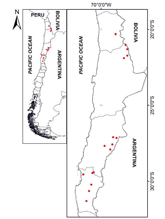
Figure 1 Arrangement of the camera traps used in this study (red points), located between Tarapaca and Coquimbo in the central-northern region of Chile. Coordinates are shown in Appendix 1.
Ecological Niche Modelling. The maximum entropy method was employed using MaxEnt 3.4.3 software (Phillips et al. 2006). This software is suitable when absent data are not reliably obtained (Stryszowska et al. 2016, Galante et al. 2018). The model was developed by delimiting South America as the area of accessibility or “area M,” even though the occurrence data points were limited to Chile. This enabled exploring niche connectivity with species previously classified as L. colocola (Nascimento et al. 2021). Based on the number of occurrences (171 coordinates. Appendix 1), the feature type “threshold features” (Elith et al. 2010) and the regularization multiplier RM=1 (Morales et al. 2017, Galante et al. 2018) were used. A detailed description of the feature types and the resulting models can be found in Phillips et al. (2006) and Phillips & Dudik (2008). A total of 50 replicates were used to obtain a robust mean model (Stryszowska et al. 2016), and the type of replicate run was bootstrap (Phillips et al. 2006). The randomized test percentage was 25. The model was developed using 100% of the records to take advantage of all available occurrence data to provide the best estimate of the ecological niche of the species and to have a better visual interpretation (Phillips et al. 2006).
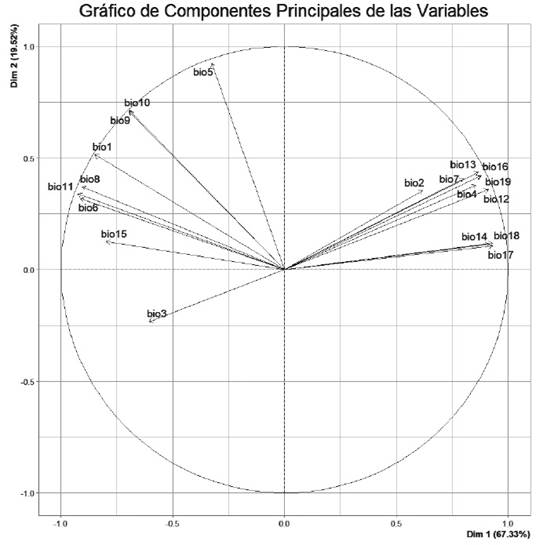
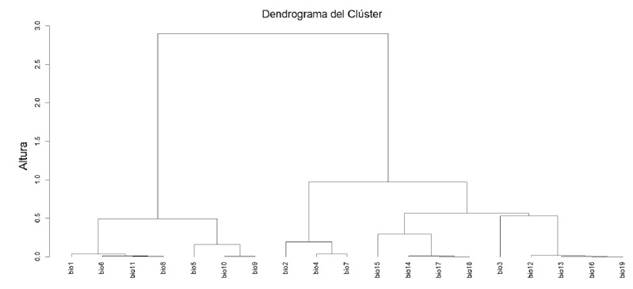
The predictive variables used in this study included the data from the 19 bioclimatic layers available in WorldClim (Fick & Hijmans 2017) and the elevation layer, following a similar approach to Nascimento et al. (2021). These variables were extracted from the coordinates of the occurrences of the species (Cuervo-Robayo et al. 2017), which allowed for characterizing the climatic or ecological niche (Mota-Vargas et al. 2019). The variables that contributed the most to the spatial-environmental variation of the species were selected using a variable clustering analysis, which helped to eliminate strongly correlated variables. This variable selection was performed with the ClustOfVar package (Chavent et al. 2012) run from R (R Core Team 2023). This analysis reduced the 19 variables to only eight: Bio1 = Annual Mean Temperature, Bio 2 = Mean Diurnal Range (Mean of monthly (max temp - min temp)), Bio 3 = Isothermality (BIO2/BIO7) (×100), Bio 4 = Temperature Seasonality (standard deviation ×100), Bio 10 = Mean Temperature of Warmest Quarter, Bio 15 = Precipitation Seasonality (Coefficient of Variation), Bio16 = Precipitation of Wettest Quarter. The resulting logistic model provided a predicted spatial probability of occurrence ranging from 0 (low) to 1 (high). The reliability of the model was evaluated using the area Under the Curve (AUC) of the receiver operating characteristic (ROC) curve (Fielding & Bell 1997). The AUC ranges from 0.5 (low discrimination) to 1 (perfect discrimination), and the general rule states that AUC values above 0.75 are considered informative (Eskildsen et al. 2013). The threshold of the ecological niche model was established with the value that allowed the incorporation of all the coordinates of the presence of the species to deal with the underestimation (Loiselle et al. 2003).
The EOO is “the area contained within the shortest continuous imaginary boundary which can be drawn to encompass all the known, inferred or projected sites of present occurrence of a taxon, excluding cases of vagrancy” (IUCN Standards and Petitions Committee 2022). It was calculated using the alpha hull method (a generalization of a convex hull), which describes the distribution area’s external shape by dividing it into several differentiated polygons (IUCN Standards and Petitions Committee 2022). Using the QGIS 3.28 software, a Delaunay triangulation was constructed using the species’ occurrence coordinates. Then, the mean length of all lines was calculated. Next, lines with lengths greater than a multiple (alpha) of the mean line length were deleted (where the product of alpha and the mean line length represents a “discontinuity distance”). The alpha value was two, as the IUCN Standards and Petitions Committee (2022) recommends. This process eliminated the lines connecting points that were relatively distant from each other. Finally, the EOO was calculated by summing the remaining triangles’ areas. This alpha hull method allows for assessing reductions in continuous declines of the EOO, reducing biases resulting from the spatial arrangement of habitat (Burgman & Fox 2003).
The AOO is a scaled metric that represents the area of suitable habitat currently occupied by the taxon. It was calculated through the occupancy of 2x2 km grids (4 km2) (IUCN Standards and Petitions Committee 2022). This ensured that the AOO estimation corresponded to the implicit scale of IUCN thresholds (IUCN Standards and Petitions Committee 2022). The formula is AOO = (number of occupied cells) x (cell area).
Threats and conservation status. To assess the impact of mining activity, the resulting area was calculated by subtracting the mining concessions layer of Chile (codes 1932 and 1983) from the niche model, EOO, and AOO. These data were obtained from the National Geology and Mining Service (2022). Furthermore, the road network layer of Chile (National Congress Library of Chile 2018) was overlaid with the niche model, EOO, and AOO to assess the potential for roadkill incidents. Finally, following the criteria set by the IUCN Standards and Petitions Committee (2022), a new conservation status was proposed for the species.
Results
The camera traps used in this study did not record the occurrence of the species. From the reviewed databases, 171 occurrence coordinates were collected (Appendix 1). The ecological niche model of L. colocola showed an area of 157310 km2 (Table 2, Figure 2). The mean training AUC for the replicate runs was 0.991 (SD = 0.00), indicating good performance. The variables that best explained the model were Bio 15 with a contribution of 41.9% (Figure 3), Bio 3 with 26.2%, and Bio 10 with 17.1%. The cut-off threshold, including all the presence coordinates, was determined using the Maximum Training Sensitivity plus Specificity Logistic Threshold, corresponding to 9.73%. The model also predicted ecological niche presence along the central-northern coast of Peru, the northern cordillera of Chile, part of Bolivia, and Argentina, Overlapping with the climatic niche models of Leopardus garleppi proposed by Nascimento et al. (2021) (Figure 2). The EOO of the species was estimated to be 46985.5 km2 (Table 2. Figure 2), while the AOO was calculated to be 630.8 km2 (Table 2).
Table 2 Areas of the ecological niche model, area of Extent of Presence (EOO), and area of Occupation (AOO), resulting after subtracting mining concessions. Additionally, the length of the road network is shown.
| Parameter | Area (km2) | Mining concessions (km2) | Resulting area (km2) | Road network (km) |
|---|---|---|---|---|
| Niche model | 157310.0 | 54100.6 | 103209.4 | 33213.3 |
| EOO | 46985.5 | 22387.1 | 24598.4 | 9765.4 |
| AOO | 630.8 | 274.3 | 356.5 | 176.0 |
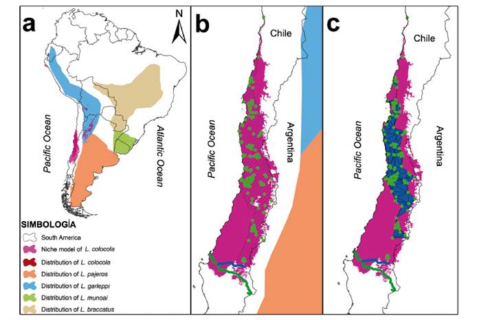
Figure 2 (a) Niche model of Leopardus colocola compared to the distribution of other species in the “pampas cat” group according to Nascimento et al. (2022). (b) Niche model of Leopardus colocola, occurrence points, and distribution proposal outlined by Castro-Pastene et al. (2023), in shaded polygon. (c) Extent of Occurrence (EOO) in blue polygon within the context of the niche model of Leopardus colocola. (b) and (c) show the Laja (blue line) and BíoBío (green line) rivers.
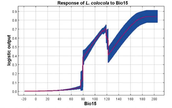
Figure 3 Predicted probability variation and mean response of the 50 replicate Maxent runs (in red), with mean values and +/- one standard deviation (in blue), depicting Bio15 (Precipitation Seasonality - Coefficient of Variation).
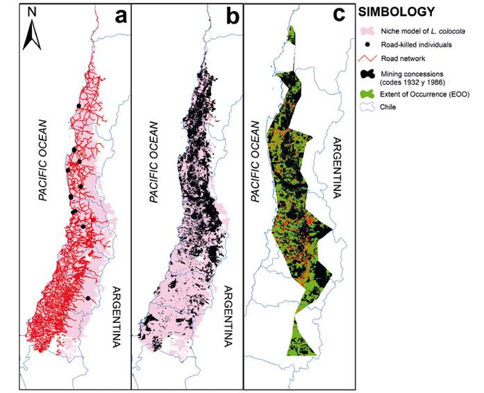
Regarding the threat posed by the road network, it has a total length of 37927.7 km within the niche model, with a densely intertwined spatial configuration mainly concentrated in the western region, leading to pronounced landscape fragmentation (Table 2, Figure 4). The mining concessions exhibited a higher concentration in the central-northern region of the niche model, covering a total area of 54100.6 km2. Exploiting these concessions implies severe fragmentation and a reduction of the niche model of 27.1%. The impact on the EOO involved severe fragmentation and a reduction of 47.7% and 43.5% on the AOO (Table 2. Figure 4). The EOO encompassed 9765.4 km of roads, with 176 km crossing the AOO.
Discussion
Ecological niche model. The findings of this study put forth a novel ecological niche model proposal, along with the expected impact of mining activities and road networks. Compared to the Nascimento et al. (2021) model, the increased number of used coordinates enabled a more robust and expanded niche prediction (Figure 1a). The development of our model coincided with that presented by Nascimento et al. (2021) on five predictive variables (Bio2, Bio3, Bio10, Bio15, and Bio17), despite using different variable selection methods. Although Nascimento et al. (2021) did not specify which variable explained their model, the ecological niche, and the probability of the occurrence of L. colocola, in this study they were primarily explained positively by the seasonality of precipitation (Bio15), followed by variations in temperature (Bio3 and Bio10). The positive relationship of species occurrence with Bio15 (Fig. 2) contrasts with the relationship found by Tirelli et al. (2021) for Leopardus munoai (the sister species of L. colocola); that is, L. munoai responded negatively to Bio15. However, this alignment with the growth stages of trees in forest habitats and their maintenance (Brienen & Zuidema 2005) suggests that the species not only inhabits desert environments but also forested ones (Castro-Pastene et al. 2023). Nonetheless, it does not support Castro-Pastene et al. (2023) hypothesis that the species avoids the humid forests around the locality of Concepción.
A limitation in potential distribution studies or ecological niche modeling is that they do not consider geographic barriers in their predictions (Cuervo et al. 2023). According to the occurrence records and the findings of this study (Figure 2), it appears that the Laja River, in together with the BíoBío River, constitutes a geographical barrier, effectively demarcating the southern limit of the species distribution as proposed by Castro-Pastene et al. (2023), even though the resulting niche model minimally exceeds this limit. Indeed, we agree with Castro-Pastene et al. (2023) that it is necessary to increase sampling efforts, particularly in areas with gaps in records, to enhance our understanding of the distribution of this species.
Conservation Status. The Criteria A, C, and D of the IUCN Red List refer to the total number of mature individuals of the assessed taxon (IUCN 2012). However, in the case of L. colocola, determining the total number of individuals is challenging due to its elusive nature (Kinnaird et al. 2003, Linkie et al. 2006). Faced with this difficulty, the Criteria B of the IUCN Red List emerges, which relates to the size of the geographic distribution area and the threats that may lead to its reduction, fragmentation, or continuous observed, inferred, or projected decline (IUCN 2012). In a more precise approach, the application of Criterion B2 by the IUCN primarily focuses on the size of the Area of Occupancy (AOO) (IUCN Standards and Petitions Committee 2022). According to our results, the AOO measured at 630.8 Km2 (Table 2) falls below one of the thresholds of Criteria B2 (AOO < 2000 km2). However, the projection of mining concessions could reduce the AOO by 56.5% as implemented (Table 2). This scenario is critical because mining production in Chile is expected to increase by 20.7% by 2030 (Cifuentes & Garay 2019). The high fragmentation of the AOO is evident and could be aggravated if we consider the 176 km of roads that currently cross it (Figure 4a. Table 2). It is important to note that one of the major threats to the species is mortality due to roadkill incidents (Guzmán-Marín et al. 2022). In fact, 12 records from this study (7%) corresponded to roadkill incidents. As a result of the fragmentation and the projected reduction of the EOO from 46985.5 km2 to 24598.4 km2 (Table 2, Figure 4c), as well as the decrease in AOO from 630.8 km2 to 356.5 km2, the species meets the criteria specified in B2ab (i, ii, iii). Consequently, it is classified as ‘Endangered’ in terms of its conservation status.
Given the proposed conservation status faced by the species, it is crucial to quantify its threats, such as dog attacks, roadkill, hunting, lack of wildlife crossings, absence of biological corridors in the face of mining development, etc. These quantifications will provide essential insights for developing a conservation plan following the Open Standards for the Practice of Conservation (Conservation Measures Partnerships 2020). This plan must be prioritized, including habitat protection, particularly regarding mining and road activities; establishing biological corridors with a medium-term vision to ensure connectivity between fragments; and emphasizing wildlife crossings to mitigate roadkill incidents. While human-wildlife conflicts involving the species remain unknown, evaluating and addressing them if they arise (coexistence) is crucial. Continued studies on the ecology and distribution of the species will also provide valuable information for making informed decisions for its protection and management. Finally, no conservation plan will be successful without working on education and awareness efforts to raise public consciousness. These general recommendations will contribute to conserving an endemic species part of Chile’s natural heritage.
Supplementary material
Supplementary material 1. Gráfico de los Componentes Principales de las Variables
Supplementary material 2. Dendrograma del Clúster
Supplementary material 3. Asignación de clústeres para cada variable
Supplementary material 4. Cargas Cuadráticas y Correlaciones de Variables Dentro de Cada Clúster
Supplementary material 5. Varianzas Explicadas por los Componentes Principales para Cada Clúster
Supplementary material 6. Puntuaciones Sintéticas para las seis de Primeras Observaciones en Cada Clúster de 170


 uBio
uBio 

