10.15381/rpb.v23i2.12427

TRABAJOS ORIGINALES

Biogeochemical validation of an interannual simulation of the ROMS-PISCES coupled model in the Southeast Pacific

Validación biogeoquímica de una simulación interanual del modelo acoplado ROMS-PISCES en el Pacífico Sudeste

 

Dante Espinoza-Morriberon ¹*, Vincent Echevin ², Jorge Tam ¹, Jesús Ledesma ¹, Ricardo Oliveros-Ramos ¹, Jorge Ramos ¹ and Carlos Y. Romero ^1,3

(1)Instituto del Mar del Perú, Esq. Gamarra y Valle s/n, Apartado 22, Callao, Perú.

(2) Laboratoire d’Océanographie et de Climatologie: Expérimentation et Analyse Numérique (LOCEAN), Institut Pierre-Simon Laplace (IPSL), UPMC/CNRS/ IRD/MNHN, 4 Place Jussieu, Case 100, 75252 Paris cedex 05, France.

(3) Universidad Nacional de Ingeniería, Facultad de Ciencias, Av. Túpac Amaru 210, Rímac, Lima

---

Abstract

Currently biogeochemical models are used to understand and quantify key biogeochemical processes in the ocean. The objective of the present study was to validate predictive ability of a regional configuration of the PISCES biogeochemical model on main biogeochemical variables in Humboldt Current Large Marine Ecosystem (HCLME). The statistical indicators used to evaluate the model were the bias, root-mean-square error, correlation coefficient and, graphically, the Taylor’s diagram. The results showed that the model reproduces the dynamics of the main biogeochemical variables (chlorophyll, dissolved oxygen and nutrients); in particular, the impact of El Niño 1997-1998 in the chlorophyll (decrease) and oxygen minimum zone depth (increase). However, it is necessary to carry out sensitivity studies of the PISCES model with different key parameters values to obtain a more accurate representation of the properties of the Ocean.

Keywords: PISCES model; HCLME; chlorophyll; dissolved oxygen; nutrients.

---

Resumen

Los modelos biogeoquímicos en la actualidad son utilizados para entender y cuantificar los principales procesos biogeoquímicos que suceden en el océano. El objetivo del presente estudio es validar estadísticamente la habilidad predictiva de una simulación del modelo biogeoquímico PISCES en reproducir la dinámica de las principales variables biogeoquímicas del Ecosistema de la Corriente de Humboldt (ECH). Para evaluar el modelo se utilizaron indicadores estadísticos: sesgo, error de la raíz del cuadrado medio, coeficiente de correlación y gráficamente el diagrama de Taylor. Los resultados muestran que el modelo es capaz de reproducir la dinámica de las principales variables biogeoquímicas (clorofila, oxígeno disuelto y nutriente), captando bien el impacto que tiene El Niño 1997-1998 en la clorofila (disminución) y profundidad de la zona mínima de oxígeno (incremento). Es necesario llevar a cabo estudios de sensibilidad del modelo PISCES usando diferentes valores de los principales parámetros para obtener una mejor representación de las propiedades biogeoquímicas del océano.

Palabras claves: modelo PISCES; ECH; clorofila; oxígeno disuelto; nutrientes.

---

Introduction

Oceanographic models are used to study several ocean processes (i.e. Kelvin waves impacts, coastal upwelling) and, in recent years, biogeochemical models have been developed to understand, quantify and predict the main biogeochemical processes and the complex dynamics between nutrients and plankton. In addition, biogeochemical models are coupled or used as forcings for High Trophic Level (HTL) models, aiming to understand ecosystem dynamics.

Intermediate complexity biogeochemical models, like NPZD type models, simulate the interaction between nitrate, phytoplankton, zooplankton and detritus (Edwards 2001, Heinle & Slawig 2013). More complex biogeochemical models like PISCES model (Aumont & Bopp 2006) or BioEBUS model (Gutknecht et al. 2013) include more variables and processes, simulating a more complete representation of the ocean biogeochemistry and plankton dynamics.

Biogeochemical models have been used in previous studies in Humboldt Current Large Marine Ecosystem (HCLME) in order to understand the climatological processes affecting the Oxygen Minimum Zone (OMZ) (Montes et al. 2014) and the climatological (Echevin et al. 2008, Albert et al. 2010) and interannual (Echevin et al. 2014) variability of phytoplankton and nutrients.

In the present study, we used statistical metrics to assess the skill of the coupled hydrodynamic and biogeochemical ROMSPISCES model using data from surveys, remote sensing and international databases.

We analyzed the climatological and interannual (1992 2008) biogeochemical variability, including the impact of El Niño 1997 ‒ 1998 event on the chlorophyll concentration and depth of the OMZ.

Material and methods

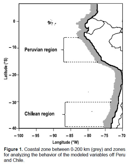
Study area.- The study area comprised the HCLME (0ºS − 40ºS and 70ºW − 100ºW). To validate the biogeochemical model, two zones were defined: a) the area off Peru within 200 km and between 06°S − 16°S; b) the area off Chile within 200 km and between 30°S − 40°S (Fig. 1). The seasons were defined as follows: summer (January − March), autumn (April − June), winter (July − September) and spring (October − December).

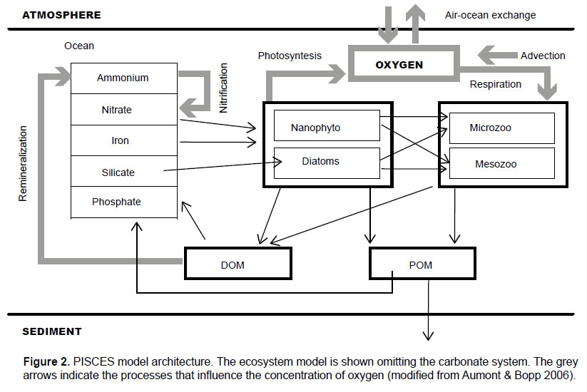
PISCES biogeochemical model.- The PISCES biogeochemical model (Pelagic Interaction Scheme for Carbon and Ecosystem Studies) simulates marine biological productivity and describes biogeochemical cycles like carbon and major nutrients in the ocean (Aumont & Bopp 2006). PISCES model assumes that phytoplankton growth depends on external concentration of nutrients and that the main nutrients in the medium follow the Redfield ratio (C:N:P ~106:16:1) (Redfield et al 1963). PISCES has 24 state variables, such as: nutrients (Phosphorus, Nitrogen, Silica and Iron), dissolved oxygen, two types of detritus (large and small), two classes of zooplankton (microzooplankton and mesozooplankton) and two classes of phytoplankton (nanophytoplankton and diatoms) (Fig. 2). Diatoms differ from nanophytoplankton in their requirements of silicates, an increased consumption of iron and higher levels of nutrient saturation due to its larger size (Echevin et al. 2008).

Model configuration.- In the present study the PISCES model is coupled to the hydrodynamical model ROMS (Regional Ocean Modeling System) (Shchepetkin & McWilliams 2005), following the coupling principles of Gruber et al. (2006), who coupled ROMS to a simpler biogeochemical model than PISCES. The physical model ROMS has been used in several previous works to simulated the dynamics of the HCLME (Penven et al. 2005, Colas et al. 2008, Montes et al. 2010, Echevin et al. 2012, Illig et al. 2014).

Our simulation covered a larger area to the north (10ºN) than the HCLME to reproduce more accurately the equatorial circulation, because surface and subsurface equatorial currents can affect the dynamics (Montes et al. 2010), oxygenation and productivity (Espinoza-Morriberón 2012) of Peruvian waters. The model spatial resolution was 1/6º with 32 sigma vertical levels (which follow the topography of the ocean floor), the output simulations were recorded of every averaged 6 days from 1992 to 2008.

Atmospheric forcings were obtained from two sources: (1) merging climatological SCOW data (Risien & Chelton 2008) with NCEP anomalies (www.ncep.noaa.gov/) for wind fields and, (2) merging COADS climatology data (Da Silva et al. 1994) with NCEP anomalies for the heat fluxes and air temperatures. For boundary conditions the outputs of the global ORCA2-PISCES physical-biogeochemical coupled model (Aumont & Bopp 2006) were used. More details about model configuration are described in Echevin et al. (2010, 2012) and Cambon et al. (2013).

Model Validation

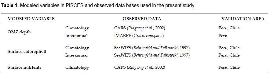
Data to validate the model.-To verify that the PISCES model represents the main spatial patterns of biogeochemical variables in the HCLME (i.e. depth of the OMZ, nutrients and surface chlorophyll), the following climatologies and interannual time series were used (Table 1):

Chemical. Oxygen and nutrients climatologies were obtained from CSIRO Atlas of Regional Seas "CARS 2009" (Ridgway et al. 2002) at a spatial resolution of 1/2º and a vertical resolution of every 5 m depth (from 0 − 200 m) and every 100 m depth (from 200 − 1000 m). Monthly series from 1992 to 2008 of the depth of the upper limit of the OMZ were obtained by merging the database of the Instituto del Mar del Peru (IMARPE) and the international database of WOD09 (García et al. 2010), following the methodology developed by Musial et al. (2011); the reader is referred to Bertrand et al. (2011) for more details about oxygen data processing.

Biological. Surface chlorophyll climatological and interannual time series was obtained from the database of the Sea-viewing Wide Field-of-view Sensor (SeaWiFS) (Behrenfeld & Falkowski 1997) at a spatial resolution of 1/12º and a monthly temporal resolution from 1997 to 2008.

All observed time series were interpolated on the model temporal resolution using the Laplace transformation method implemented in the FERRET program (http://ferret.pmel. noaa.gov/Ferret) to make comparisons between model and observations.

Data analysis.- Goodness of fit between observed and simulated data was measured using the following statistical indicators (Vichi and Masina 2009, Lehmann et al. 2009):

Bias (S), which reflects the overestimation (positive) or underestimation (negative) of a simulation:

S = 1/n ∑(M – O) ……………(Eq.1)

Where n represents the number of pairs between observed (O) and modeled (M) data by time each bin. However it is necessary to keep in mind that positive and negative deviations in the model tend to cancel, so that the bias would represent the persistence of a difference between the modeled (M) and observed (O) values.

Root mean square error (RMSE), reflects whether the modeled values differ in magnitude from the observed values, so that a small RMSE would indicate good agreement between modeled and observed values:

RMSE= √((∑(M – O)^2 )/n)……………(Eq.2)

Correlation coefficient, allows us to assess how strongly the temporal variations of the modeled and the observed values are related:

ρ(M,O)= cov(M,O)/(σ_M σ_O )……………(Eq.3)

Where cov (M, O) is the covariance between the time series of M and O, and σ_M σ_O are the standard deviations of M and O respectively.

In addition, Taylor diagrams (Taylor 2001) were used to evaluate the goodness of fit of the model: 1) between areas (off Peru and Chile), and 2) between temporal variations (climatological and interannual). Taylor diagram integrates the RMSE, the correlation coefficient and the standard deviation in a single diagram, to compare the fields that are tested (coming from one or more models) and a reference field (representing the "truth" or the observed field).

Results and discussion

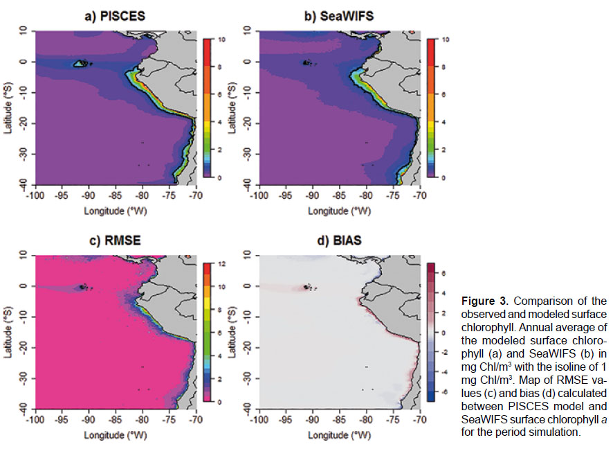
Surface chlorophyll.- SeaWIFS interannual satellite data (1997-2008) were interpolated on the model spatial resolution (~18 km) and the climatologies (for satellite and simulated data) were calculated between the years 2000-2008 to reduce the effect of the strong 1997-98 "El Niño". Figure 3 (a and b) shows that the simulation represents adequately the average spatial distribution of surface chlorophyll observed, reproducing larger chlorophyll values near the coast. In addition, the area of greatest productivity of the HCLME (Northern Central Peru) and the simulated distribution of the 1 mg Chl/m³ isoline, used as a proxy to define the upwelling area (Nixon & Thomas 2001), follows the annual pattern observed in SeaWiFS data. The high productivity observed off the Northern Center Peruvian region could be generated by the widening of the continental shelf in this area, which would provide a high amount of iron to the water column. The iron is generally a key limiting element for phytoplankton (Bruland et al. 2005).

Goodness of fit indicators validated the model within the study area: within 200 km of the coast in Peruvian area, mean values of RMSE around 3.2 mg Chl/m³ and a mean positive bias of ~+2.5 mg Chl/m³ (Fig. 3c and 3d) were observed; furthermore, in the whole modelling region RMSE values mainly fluctuated between 0 at 0.5 mg Chl/m³ and bias values between -0.1 to 0.1 mg Chl/m³. The overestimation of the simulations compared to the observed pattern could be influenced by the presence of clouds near the coast off Peru that could have masked some phytoplankton blooms. Another explanation for the model overestimation would be the lack of two-way coupling between PISCES and high trophic level model (to connect large zooplankton to top predators), which could influence phytoplankton mortality (Traver & Shin 2010). Also, a slightly positive bias was observed in the equatorial upwelling, which has also been observed by Albert et al. (2010), possibly because the model overestimate the equatorial upwelling.

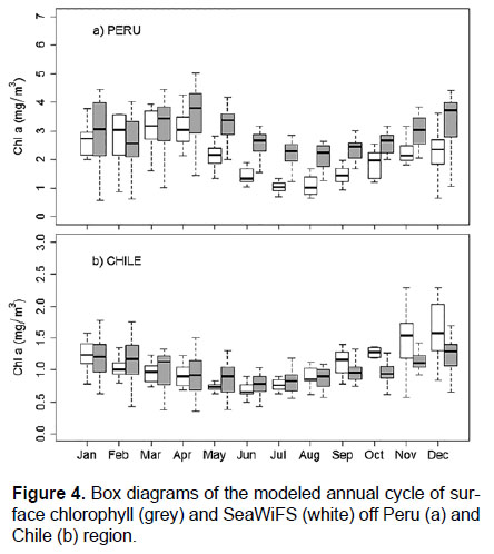
The annual cycle of surface chlorophyll within 200 km was acceptably reproduced by the model off the coasts of Peru and Chile compared to the SeaWiFS data (from here, satellite values will be given in parentheses). Seasonality off Peru had larger amplitude than in Chile. The mean seasonal chlorophyll concentration presented highest values off Peru during the summer and autumn months with 3.5 (3.2) mg Chl/m³ and lower values during winter with 2.5 (1.2) mg Chl/m³, while off Chile, highest values were observed during spring and summer with 1.2 (1.5) mg Chl/m³ and lower values during winter with 0.9 (0.92) mg Chl/m³ (Fig. 4). Within the coastal area off Peru, overestimation of simulations compared to SeaWIFS was also observed by Echevin et al. (2008) during all climatological months (~+1 mg Chl/m³) and by Albert et al. (2010) especially during winter, who mentioned that it could be due to the reduced availability of satellite data near the coast by the presence of clouds in this period. In Chile, this overestimation is weaker than off Peru due to fewer clouds in this area (Demarcq, pers. comm.).

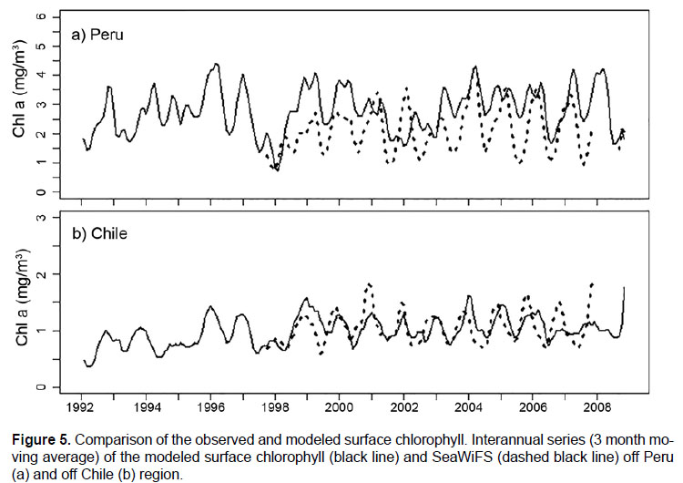
In figure 5 we can observe that the model reproduced the interannual pattern of SeaWIFS chlorophyll data off Perú; however with more productive values in most of the studied period (1997 to 2008) with the exception of the summer months; furthermore off Chile the simulation also followed adequately the interannual pattern and the magnitude of SeaWIFS values. The correlation between observations and simulations was 0.56 (Peru) and 0.43 (Chile) (p < 0.05 for both correlations). Echevin et al. (2014) also found an interannual overestimation compared to SeaWIFS off Peru (almost the same magnitude as our simulation) and mentioned that cloud presence makes difficult the validation process. The effects of El Niño were captured by the model showing decreased values of chlorophyll (0.6 mg Chl/m³) during the years 1997/1998 off Peru. The decreased level of chlorophyll during "El Niño" along Peruvian coast is caused by poor waters advected from Equator region and by more frequency of downwelling Kelvin waves that produce the deepening of the nutricline (Echevin et al. 2014).

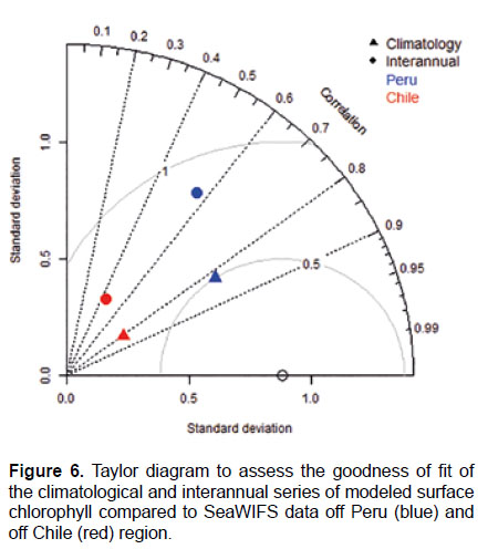
Taylor diagram (Fig. 6) comparing climatological and interannual variations of chlorophyll in the areas off Peru and Chile within 200 km of the coast showed that the model has a better goodness of fit off Peru than off Chile; and in addition, goodness of fit was better for the chlorophyll seasonal cycle than for the interannual variation in both areas.

Surface nutrients.-Nutrients climatology from CARS was also interpolated on 18 km resolution grid and simulated nutrients climatology was calculated for the period 1992 – 2008 to be comparable with CARS data, taking into account about 50 years of observed data.

On annual average, the model represented adequately in the Peruvian region the spatial distribution of observed nutrients, with higher concentrations near the coast; however, for the three nutrients used in the present study (nitrates, phosphates and silicates) a positive bias of the concentrations was obtained for the most study area (not shown). The overestimation of nutrients in the PISCES model compared to observations, although with less magnitude in our simulations, has also been observed by Echevin et al. (2008) and Albert et al. (2010), who explained that it could be due to high concentrations of nutrients in the boundary conditions and that the upwelling of nutrients during winter would be stronger in the model than in reality. In the configuration of Echevin et al. (2014), nitrate and phosphate are also overestimated (+1 y +0.3 µmol/L, respectively) and silicate is underestimated (~-1.5 µmol/L) compared to IMARPE data.

The seasonal cycle showed more nutrients during winterspring possibly due to more vertical mixing; and less concentration during summer, when there is more nutrient consumption by phytoplankton. This variability is also observed by Calienes et al. (1985).

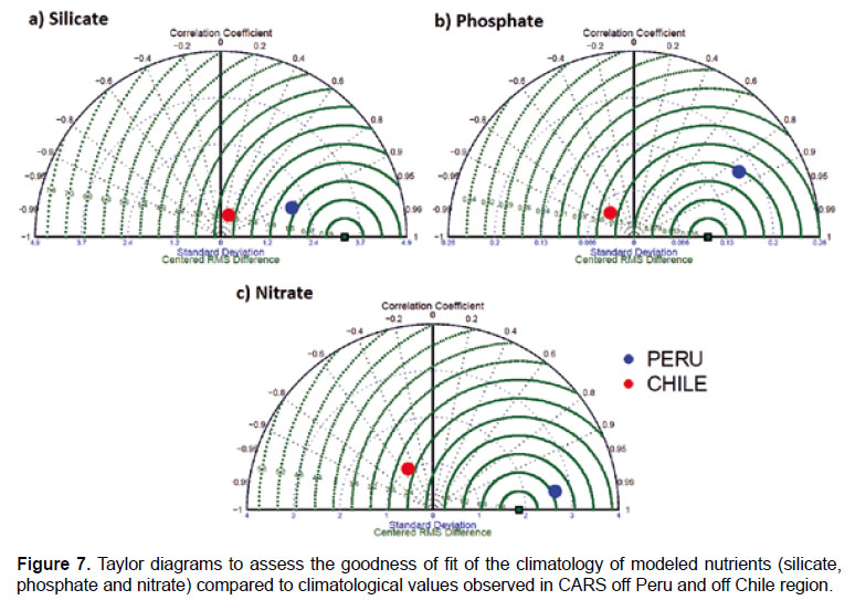
In Figure 7 Taylor diagram indicated that modelled nutrients had a higher goodness of fit off Peru than off Chile.

Depth of the OMZ.- The depth of the OMZ in this study is defined as the depth at which the concentration of dissolved oxygen is 88 µmol/kg (2 mL/L), because it is the concentration limit for the optimal development of pelagic species (Bertrand et al. 2011). Dissolved oxygen data from CARS on surface and vertical levels were interpolated to 18 km.

The model represented adequately the spatial distribution of the depth of the OMZ, with a shallower OMZ near the ocean off Peru, as observed in CARS (Fig. 8a and 8b). The presence of a stronger and shallower OMZ off Peru could be due to: 1) a high rate of remineralization influenced by high primary productivity, 2) a lack of ventilation due to the presence of a strong pycnocline that keeps subsurface waters isolated from the atmosphere, plus deoxygenation of equatorial currents that are the main source of oxygen in this zone (Stramma et al 2010.) and; 3) the long residence time of the waters with a cumulative reduction of oxygen (Czeschel et al. 2011).

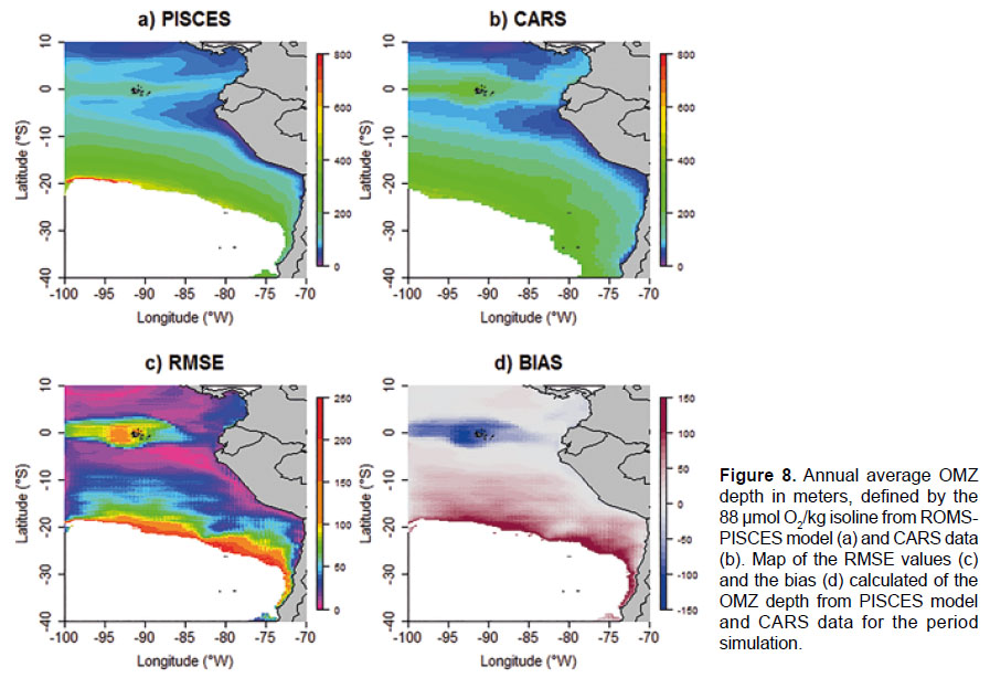
RMSE values fluctuated between 0 to 50 µmol/kg and the bias between -20 to 40 µmol/kg. Lower values of RMSE and bias were obtained off Peru; however, an underestimation in the equatorial zone and an overestimation at the south of the HCLME (between 20ºS to 40ºS) of the depth of the OMZ was observed (Fig. 8c and 8d). The greatest differences observed at the equator and at the south of the HCLME could be due to a slight lack of representativeness of the intensities of the currents in the boundary conditions used in the configuration of our simulation in these areas, which could lead to less oxygen flow in the equatorial zone and greater oxygen flow off Peru (Espinoza-Morriberón 2012).

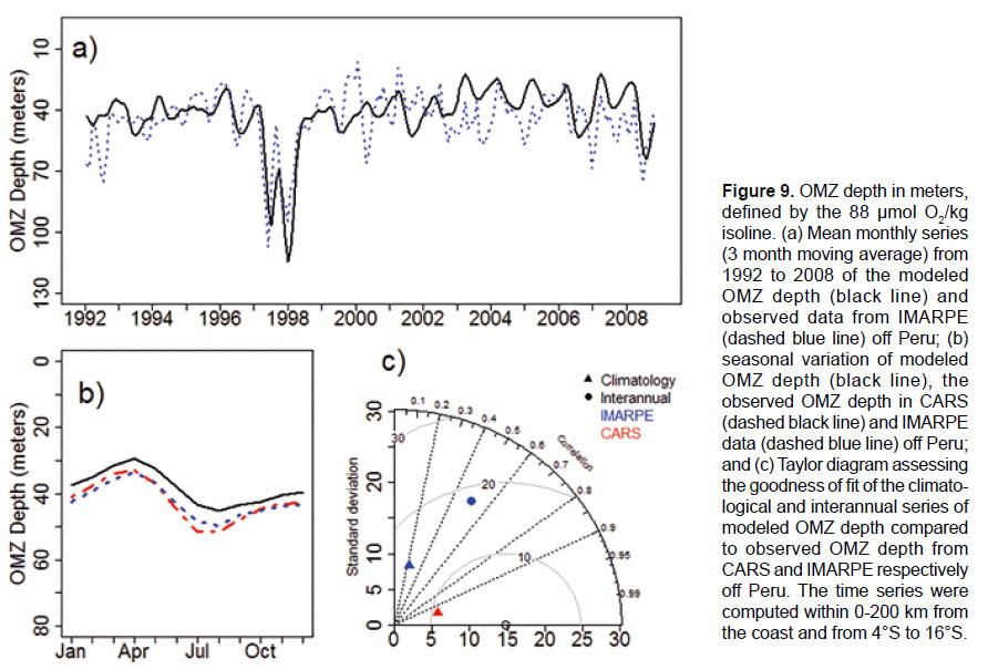
The model represented adequately the seasonal signal of the OMZ upper limit depth off Peru; however the values from CARS and IMARPE were underestimated on average throughout the year. The OMZ is shallower during the summer-autumn and deeper during winter-spring (Fig. 9b), probably related to: (a) during winter the vertical mixing is stronger due to more wind intensity and (b) during autumn after high phytoplankton biomass dying, organic matter is consumed by bacteria during the remineralization process with a consequently high consumption of dissolved oxygen (Libes 1992, Paulmier et al. 2006). Interannually, the model reproduced the oxygenation events during "El Niño" (shallower OMZ) and the observed dissolved oxygen from IMARPE; however, it presented some deficiencies in following the interannual pattern (Fig. 9a). The correlation between simulations and observations off Peru was 0.42 (p<0.05). The deepening of the OMZ during "El Niño" could be due to the impact of Kelvin waves and the intrusion of surface tropical waters rich in oxygen and poor in nutrients. Taylor diagram (Fig. 9c) showed for OMZ depth that correlation with IMARPE data was higher for the climatology than for interannual variations.

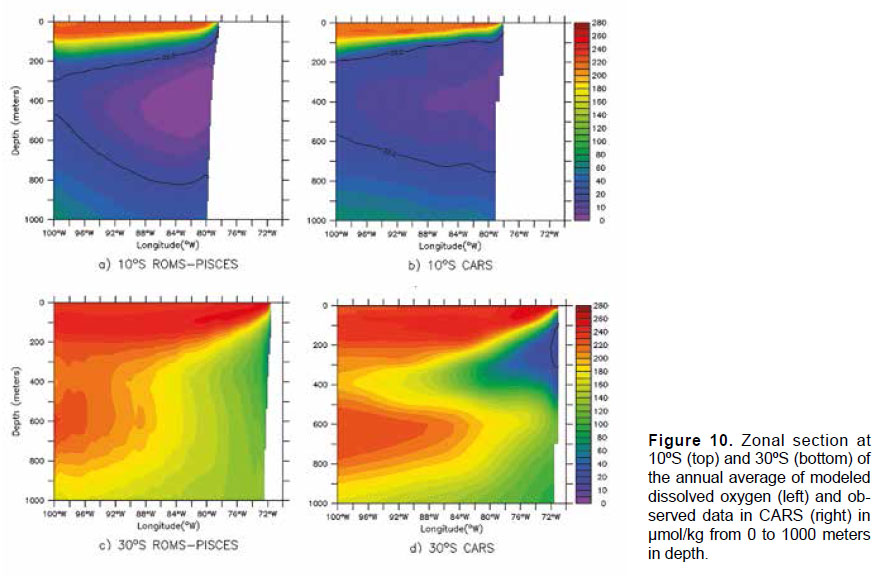
In other hand, vertically the model reproduced relatively well the vertical structure of dissolved oxygen off Peru and Chile compared to CARS data (Fig. 10); however, the modeled OMZ off Peru tend to be larger than CARS OMZ. The greater intensity of the OMZ in front of Peru is the result of high primary production reproduced in the model; another aspect to consider is the values of the remineralization of dissolved organic carbon (0.3 d⁻¹) and nitrification (0.05 d⁻¹) rates used in our configuration that influence oxygen consumption in the model (Espinoza-Morriberón 2012). Sensitivity studies of PISCES model at different values of these parameters need to be explored in the future. CARS climatological data base could also present deficiencies in accurately represent the values within the OMZ, because they are based on World Ocean Atlas (WOA) data, which tend to overestimate the O₂ within the OMZ due to various factors such as: positive biases in old measurements, interpolation artifacts and the effects of variability in ocean circulation (Bianchi et al. 2012).

Coupled ROMS-PISCES model has been validated in other works for the Peruvian region, explaining the interactions of phytoplankton and nutrients in climatological (Echevin et al. 2008, Albert et al. 2010) and interannual (Echevin et al. 2014) mode; however in the present configuration we reproduced the interannual dynamics of biogeochemical variables on a longer period (17 years) and during the occurrence of an extreme El Niño (1997−1998). On the other hand, the dissolved oxygen dynamics was studied and we could observe El Nino impact on it.

Conclusions

The present configuration of the ROMS-PISCES model reproduced adequately the dynamics of the main biogeochemical variables (chlorophyll, nutrients and the depth of the oxycline) in the HCLME. The model showed a very productive system near the coast and the seasonal cycles of chlorophyll, nutrients and depth of the OMZ were acceptably reproduced. Regarding the interannual signal, the model captured well the decrease in chlorophyll concentration and the increase in OMZ depth produced by "El Niño"; however we have to keep in mind that the model represented the climatological variations better than the interannual variations.

It is noteworthy that this study presents one of the first attempts to reproduce the dynamics of biogeochemical variables in the HCLME (Echevin et al. 2008, Albert et al. 2010, Echevin et al. 2014, Montes et al. 2014). However, the present configuration of the model still has several problems to be solved. It is necessary to conduct sensitivity analysis of the model with different boundary conditions, forcings and different values of key parameters of the PISCES model, such as rates of remineralization and nitrification, among others.

Acknowledgements

We acknowledge Christophe Hourdin for providing model configurations and running the simulation performed within the PEPS project, Carlos Quispe from LMOECC (IMARPE) for their valuable comments on the statistical analysis. This work was published with the support of IRD and the JEAI EMACEP (Ecología Marina Cuantitativa del Ecosistema de Afloramiento Peruano) and the LMI DISCOH (Dinamica de Sistema de Corriente de Humboldt).

Literature cited

Albert A., V. Echevin, M. Levy, et al. 2010. Impact of the nearshore wind stress curl on coastal circulation and primary productivity in the Peru upwelling system. Journal of Geophysical Research 115:C12033. doi: http://dx.doi.org/10.1029/2010JC006569.         [ Links ]

Aumont O. & L. Bopp. 2006. Globalizing results from ocean in situ iron fertilization studies. Global Biogeochemical Cycles 20:GB2017. doi: http://dx.doi.org/10.1029/2005GB00259.         [ Links ]

Behrenfeld M. & P. Falkowski. 1997. Photosynthetic rates derived fromsatellite-based chlorophyll concentration. Limnology and Oceanography 42(1):1-20. doi: http://dx.doi.org/10.4319/lo.1997.42.1.0001.         [ Links ]

Bertrand A., A. Chaigneau, S. Peraltilla, et al. 2011. Oxygen: Afundamental property regulating pelagic ecosystem structure in the coastal southeastern Tropical Pacific. PLoSOne 6(12):e29558. doi: http://dx.doi.org/10.1371/annotation/891b6bd0-185f-4f5f-9f0c-d2408a31f7f4.         [ Links ]

Bianchi D., J.P. Dunne, J.L. Sarmiento, et al. 2012. Data-based estimates of suboxia, denitrification, and N₂O production in the ocean and their sensitivities to dissolved O₂. Global Biogeochemical Cycles 26:GB2009. doi: http://dx.doi.org/10.1029/2011GB004209.         [ Links ]

Bruland, K., E. Rue, G. Smith, et al. 2005. Iron, macronutrients and diatom blooms in the Perú upwelling regime: brown and blue waters of Peru. Marine Chemestry 93: 81-103. doi: http://dx.doi.org/10.1016/j.marchem.2004.06.011.         [ Links ]

Calienes R., O. Guillén & N. Lostaunau. 1985. Variabilidad espacio-temporal de clorofila, producción primaria y nutrientesfrente a la costa peruana. Boletin del Instituto del Mar del Perú - Callao 10:1-44.         [ Links ]

Cambon G., K. Goubanova, P. Marchesiello, et al. 2013. Assessing the impact of downscaled atmospheric winds on a regional ocean model simulation of the Humboldt system. Ocean Modelling 65:11-24. doi: http://dx.doi.org/10.1016/j.ocemod.2013.01.007.         [ Links ]

Colas F., X. Capet, J. C. McWilliams, et al. 2008. 1997–1998 ElNino off Peru: A numerical study. Progress in Oceanography 79:138–155. doi: http://dx.doi.org/10.1016/j.pocean.2008.10.015.         [ Links ]

Czeschel R., L. Stramma, F.U. Schwarzkopf, et al. 2011. Mid depth circulation of the eastern tropical South Pacificand its link to the oxygen minimum zone. Journal of Geophysical Research 116: C01015. doi: http://dx.doi.org/10.1029/2010JC006565.         [ Links ]

Da Silva A.M., C.C. Young & s. Levitus. 1994. Atlas of surface marinadata 1994. Technical report, Natl. Oceanogr. And Atmos. Admin. Silver Spring Md.         [ Links ]

Echevin V., O. Aumont, J. Ledesma, et al. 2008. The seasonal cycle of surface chlorophyll in the Peruvian upwelling system: A model study. Progress in Oceanography 79: 167-176. doi: http://dx.doi.org/10.1016/j.pocean.2008.10.026.         [ Links ]

Echevin V., K. Goubanova, B. Dewitte, et al. 2012. Sensitivity of the Humboldt Current system to global warming: a downscalingexperiment of the IPSL-CM4 model. Climate Dynamics38(3-4):761-774. doi: http://dx.doi.org/10.1007/s00382011-1085-2.         [ Links ]

Echevin V., A. Albert, M. Lévy, et al. 2014. Intraseasonal variability of nearshore productivity in the Northern Humboldt Current System: The Role of coastal trapped waves. ContinentalShelf Research 73: 14-30. doi: http://dx.doi.org/10.1016/j.csr.2013.11.015.         [ Links ]

Echevin, V. 2010. Peru Ecosystem Projection Scenarios. ANR. On line: https://skyros.locean-ipsl.upmc.fr/~peps/        [ Links ]

Edwards A.M. 2001. Adding detritus to a nutrient–phytoplanktonzooplankton model: a dynamical-systems approach. Journalof Plankton Research 23(4): 389-413. doi: http://dx.doi.org/10.1093/plankt/23.4.389.         [ Links ]

Espinoza-Morriberón D. 2012. Impacto de la circulación ecuatorial en la zona mínima de oxígeno presente en el norte del Ecosistema de la Corriente de Humboldt. Thesis to obtain the degree of Master in Marine Sciences. Unidad de Postgrado Víctor Alzamora. Facultad de Ciencia y Filosofía. Universidad Peruana Cayetano Heredia, Lima. 115 pp.         [ Links ]

Lehmann M.K., K. Fennel & R. He 2009. Statistical validation of a 3-D bio-physical model of the western North Atlantic. Biogeosciences 6: 1961–1974. doi: http://dx.doi.org/10.5194/bg-6-1961-2009.         [ Links ]

Garcia H.E., R.A. Locarnini, T.P. Boyer, et al. 2010. World Ocean Atlas 2009, Volume 3: Dissolved Oxygen, Apparent OxygenUtilization, and Oxygen Saturation. S. Levitus, Ed. NOAA Atlas NESDIS 70, U.S. Government Printing Office, Washington, D.C., 344 pp.         [ Links ]

Gruber N., H. Frenzel, S.C. Doney, et al. 2006. Eddy-resolving simulation of plankton ecosystem dynamics in the California Current System. Deep Sea Research 1(53): 1483-1516. doi:http://dx.doi.org/10.1016/j.dsr.2006.06.005.         [ Links ]

Gutknecht E., I. Dadou, B. Le Vu, et al. 2013. Coupled physical/biogeochemical modeling including O2-dependent processes in Eastern Boundary Upwelling Systems: Application inthe Benguela. Biogeosciences 10: 3559–3591. doi: http://dx.doi.org/10.5194/bg-10-3559-2013.         [ Links ]

Heinle A. & Slawig T. 2013. Internal Dynamics of NPZD type ecosystem models. Ecological Modelling 254: 33 – 42. doi: http://dx.doi.org/10.1016/j.ecolmodel.2013.01.012.         [ Links ]

Illig S., B. Dewitte, K. Goubanova, et al. 2014. Forcing mechanisms ofintraseasonal SST variability off central Peru in 2000-2008. Journal of Geophysical Research Oceans 119(6):3548-3573.doi: http://dx.doi.org/10.1002/2013JC009779        [ Links ]

Libes S. 1992. Introduction to Marine Biogeochemistry. John Wiley & Sons. Inc. Nueva York. 734 pp.         [ Links ]

Montes I., F. Colas, X. Capet, et al. 2010. On the pathways of the equatorial subsurface currents in the eastern equatorial Pacific and their contributions to the Peru Chile Undercurrent. Journal of Geophysical Research 115: C09003. doi: http://dx.doi.org/10.1029/2009JC005710.         [ Links ]

Montes I., B. Dewitte, E. Gutknecht, et al. 2014. High-resolution modeling of the Eastern Tropical Pacific oxygen minimum zone: Sensitivity to the tropical oceanic circulation, Journal of Geophysical Research Oceans. 119. doi: http://dx.doi.org/10.1002/2014JC009858.         [ Links ]

Musial J.P., M.M. Verstraete & N. Gobron. 2011. Comparing the effectiveness of recent algorithms to fill and smooth incomplete and noisy time series. Atmospheric Chemistry andPhysics 11: 14259–14308. doi: http://dx.doi.org/10.5194/acpd-11-14259-2011        [ Links ]

Nixon S & A. Thomas. 2001. On the size of the Peru upwelling ecosystem. Deep Sea Research I 48: 2521–2528. doi: http://dx.doi.org/10.1016/S0967-0637(01)00023-1.         [ Links ]

Paulmier A, D. Ruiz-Pino, V. Garçon, et al. 2006. Maintaining of the Eastern South Pacific Oxygen Minimum Zone (OMZ) offChile. Geophysical Research Letter 33: L20601. doi: http://dx.doi.org/10.1029/2006GL026801.         [ Links ]

Penven P., V. Echevin, J. Pasapera, et al. 2005. Average circulation, seasonal cycle, and mesoscale dynamics of thePeru Current System: A modeling approach. Journal ofGeophysical Research 110: C10021. doi: http://dx.doi.org/10.1029/2005JC002945.         [ Links ]

Redfield A.C., B.H. Ketchum & F.A. Richards. 1963. The influence of organisms on the composition of the sea-water. En: Hill M.N. (Eds.). Interscience 2: 26-77.         [ Links ]

Ridgway K.R., J.R. Dunn & J.L. Wilkin. 2002. Ocean interpolation by four-dimensional least squares-Application tothe waters around Australia. Journal of Atmospheric and Oceanic Technology 19(9):1357-1375. doi: http://dx.doi.org/10.1175/1520-0426(2002)019<1357:OIBFDW>2.0.CO;2.         [ Links ]

Risien C.M. & D.B. Chelton. 2008. A Global Climatology ofSurface Wind and Wind Stress Fields from Eight Yearsof QuikSCAT Scatterometer Data. Journal of Physical Oceanography 38: 2379-2413. doi: http://dx.doi.org/10.1175/2008JPO3881.1.         [ Links ]

Shchepetkin A.F. & J.C. McWilliams. 2005. The regional oceanic modeling system: a split-explicit, free-surface, topography-following-coordinate ocean model. Ocean Modelling 9: 347–404.doi: http://dx.doi.org/10.1016/j.ocemod.2004.08.002.         [ Links ]

Stramma L., G. Johnson, E. Firing, et al. 2010. Eastern Pacific oxygen minimum zones: Supply paths and multidecadal changes. Journal of Geophysical Research 115:C09011. doi: http://dx.doi.org/10.1029/2009JC005976.         [ Links ]

Taylor K.E. 2001. Summarizing multiple aspects of model performancein a single diagram. Journal of Geophysical Research 106: 7183–7192. doi: http://dx.doi.org/10.1029/2000JD900719        [ Links ]

Traver M. & Y.J. Shin. 2010. Spatio-temporal variability in fishinduced predation mortality on plankton: A simulationapproach using a coupled trophic model of the Benguela ecosystem. Progress in Oceanography 84(1-2):118-120. doi:http://dx.doi.org/10.1016/j.pocean.2009.09.014        [ Links ]

Vichi M. & S. Masina. 2009. Skill assessment of the PELAGOS global ocean biogeochemistry model over the period1980–2000. Biogeosciences 6: 2333–2353. doi: http://dx.doi.org/10.5194/bg-6-2333-2009.         [ Links ]

 

* Corresponding author

Email Dante Espinoza-Morriberon: despinoza@imarpe.gob.pe

Email Vincent Echevin: vincent.echevin@locean-ipsl.upmc.fr

Email Jorge Tam: jtam@imarpe.gob.pe

Email Jesús Ledesma: jledesma@imarpe.gob.pe

Email Ricardo Oliveros-Ramos: ricardo.oliveros@gmail.com

Email Jorge Ramos: jramos@imarpe.gob.pe

Email Carlos Y. Romero: cromero@imarpe.gob.pe

 

 

Información sobre los autores:

DEM redactó el trabajo y analizó los datos. VE y ROR analizaron los datos. JTM redactó el trabajo. JLR y JRF ayudaron en la recolección de datos. CRT contribuyó en la discusión en el trabajo. 

Los autores no incurren en conflictos de intereses.

Fuentes de financiamiento: JEAI EMACEP (Ecología Marina Cuantitativa del Ecosistema de Afloramiento Peruano) y LMI DISCOH (Dinamica de Sistema de Corriente de Humboldt).

 

Presentado: 31/07/2015

Aceptado: 08/06/2016

Publicado online: 27/08/2016