


Serviços Personalizados
Journal

Artigo
 texto em
  Inglês (pdf)
 Artigo em XML
 Referências do artigo
 Enviar este artigo por email
Indicadores
-
 Citado por SciELO
Links relacionados
-
 Similares em
SciELO
Similares em
SciELO
Compartilhar

 Permalink
Industrial Data
versão impressa ISSN 1560-9146versão On-line ISSN 1810-9993
Ind. data vol.26 no.1 Lima jan./jun. 2023
http://dx.doi.org/10.15381/idata.v26i1.23717
Systems and Information Technology
Application of a Discrete-Event Simulation Model to Improve the Productivity of the Production Process in a Manufacturing Company

1 Industrial engineer from Universidad Nacional Mayor de San Marcos (UNMSM). Currently working as an independent consultant (Lima, Peru). E-mail: ovasal@gmail.com
2 Industrial engineer and PhD in Industrial Engineering from UNMSM. Currently working as professor at the School of Industrial Engineering of UNMSM (Lima, Peru). E-mail: pprosalesl@gmail.com
In this paper, we introduce a simulation model using ProModel simulation software designed to propose and evaluate improvements to increase the productivity of the production process of a manufacturing company while helping to achieve the company’s objectives. The study begins with the model conceptualization, explaining the functioning of the company’s production process and detailing the transactions used in the operations. The model layout is then presented, containing the different locations, entities, and resources provided by the production process. Finally, the results of the model are transcribed with the new values of the variables that intervene in the process for comparison with the current ones to determine the conclusions of productivity improvement.
Keywords: simulation; ProModel; discrete event; productivity.
INTRODUCTION
The use of system simulation for the solution of real-time problems is becoming increasingly frequent due to the appearance of new tools that try to perfect it until reaching a remarkable level of acceptance. Manufacturing systems simulation aims to understand the operation of the business production process to provide various scenarios that show possible improvements, thus increasing the productivity of the production process, which is the aim of this research study.
Systems Simulation
According to Arnold and Osorio (1998), systems theory is a systematic and scientific approximation and representation of reality. Naylor et al. (1991) states that systems simulation is a numerical technique performed on digital computers that requires specific mathematical logic models to describe the behavior of a business or economic system or some of its components during extended periods of real-time. In addition, Fishman (1978) states that system simulation on a computer provides a method for analyzing the behavior of a system. Systems simulation is applied in all cases to provide possible solutions to the problems posed.
Methods Engineering
According to Palacios (2016), methods engineering involves the study of product development processes, service provision, and time-motion studies. Niebel and Freivalds (2009) also state that methods engineering involves the analysis at two different times during product development. First, method engineers are responsible for designing and developing the work centers, and, second, the same engineers must constantly study the work centers in order to find better ways to produce the products and improve their quality. In turn, Sellie (2006) stress that time standards are used to determine the time required by a skilled worker to perform a specific task at a normal pace, according to a specific method. On the basis of these definitions, the premise that the application of methods engineering increases the productivity of the production process of a manufacturing company originates.
Discrete-Event Simulation
Discrete-event simulation research has been conducted throughout the history of systems simulation. For instance, Cevallos et al. (2013) proposed a sequence of steps to build a discrete simulation model for the automotive service industry, as most companies regard simulation as an isolated element of the models currently used within the manufacturing field for problem-solving and improvement. The initiative to develop a model that integrates simulation and the core elements of project management was studied based on the experience gained from implementing discrete simulation models and on various theoretical references previously reviewed.
Similarly, Jiménez and Gómez (2014) developed a simulation model to evaluate and recommend improvements in a human consumption food distribution center. The quality of the service provided by the company, the response time in reception and dispatch, and operating costs were used as indicators to measure the system’s performance. A series of experiments were conducted with the model, such as the distribution of the warehouse floor layout, and some changes in the reception and dispatch processes, thus obtaining a configuration that increases the performance of the system under study by approximately 40%. Forero-Páez and Giraldo (2016) report the results obtained using a simulation model of a bicycle manufacturing process in an industrial engineering course. Students learn about the main cause-effect relations in such processes by interacting with the model. Such interaction occurs through spreadsheets, where students assign deterministic or random values to a set of decision variables or causes, including operating times, raw material purchase schedule, and preventive or corrective maintenance scheduling judged appropriate by the students to meet a defined level of bicycle demand and the use of production capacity, which are the dependent variables.
Problem Formulation
To what extent does productivity increase in a manufacturing company based on a discrete event simulation?
The general objective expresses the overall problem intended to be addressed by any research. A general statement of the problem and the idea contained in the title of the research are therefore required. According to Merino et al. (2009), every research project should first specify the objectives. The general objective of this research is to find a solution to the problem of low productivity by implementing a discrete simulation model to improve the productivity of the production process of the manufacturing company.
The purpose of this study is to contribute with some acquired knowledge to enrich the already existing theory. Furthermore, it intends to corroborate that methods engineering together with systems simulation can be used as a tool to improve the production process, allowing for sound decision-making to increase productivity in an increasingly competitive market. In this regard, our research objective is to determine to what extent the productivity of a manufacturing company is increased based on a discrete simulation. The study was conducted between January 2018 and January 2019, and the samples were collected from the plant during the production process of spring mattresses.
METHODOLOGY
According to Iglesias and Cortés (2004), methodology is the science that explains the efficient management of a given process to achieve the desired results; its objective is to provide the strategy to be followed during the development of the process. Consequently, it is important to take advantage of the benefits of discrete-event simulation and use it as a tool to design management models through a series of successive stages of the entire production process to achieve the desired result. This will be the basis for a new strategy for decision-making to reach the objective set.
Hernández et al. (2014) states that research design development is the meeting point between the conceptual phases of the research process, such as the formulation of the problem, the development of the theoretical perspective and the hypotheses, and the subsequent more functional stages. This research follows a pre-experimental design because it studies the behavior of a treatment group that is randomly chosen, and a measurement is made before and after the stimulus. Likewise, the research level is explanatory because it explains the effects that related variables have when some variations are made. The research approach is quantitative since it uses data collection to demonstrate the validity of a hypothesis. The population is composed of all the company’s processes, which are analyzed during the development of the research work, and the sample consists of the company’s spring mattress production process.
The structure of the model to be simulated using to ProModel software is also a crucial factor in the decision-making process. During simulation planning, the steps to be followed should be mentioned. Similar to all classical models, the problem is formulated, data is collected, the model is designed and built, and, finally, the results are analyzed.
RESULTS
Data Collection
According to Hernández et al. (2014), data collection involves conducting a detailed plan of techniques that lead to unifying data for a specific purpose. Thus, the data collected are the results of a series of observations made over several days, perfected to obtain the expected results. For Behar (2008), data collection refers to the use of a wide variety of techniques and tools to develop information systems. Table 1 shows the time noted down for each workstation in the production process, following the sampling.
Table 1 Record of Actual Observations at Workstations Expressed in Seconds.
| Cycle | Innerspring | Clinching | Upholstery | Quilting | Closing | Packing |
|---|---|---|---|---|---|---|
| 1 | 330 | 184 | 216 | 216 | 186 | 132 |
| 2 | 324 | 190 | 225 | 222 | 192 | 126 |
| 3 | 372 | 184 | 210 | 228 | 150 | 144 |
| 4 | 366 | 190 | 216 | 222 | 186 | 132 |
| 5 | 330 | 184 | 180 | 216 | 180 | 126 |
| 6 | 318 | 220 | 228 | 213 | 198 | 132 |
| 7 | 360 | 190 | 180 | 228 | 186 | 138 |
| 8 | 366 | 220 | 210 | 210 | 192 | 144 |
| 9 | 372 | 226 | 216 | 180 | 180 | 132 |
| 10 | 360 | 184 | 228 | 222 | 198 | 126 |
| 11 | 327 | 218 | 222 | 222 | 186 | 132 |
| 12 | 333 | 214 | 219 | 219 | 180 | 126 |
| Average | 346.50 | 200.33 | 212.50 | 216.50 | 184.50 | 132.50 |
Source: Prepared by the authors.
The number of observations required was determined based on the 12 observations listed in Table 1. Out of the 12 cycles noted, the first 10 measurements made at each of the stations of each cycle were preliminary taken; the observed times (TO) were computed; the ranges (R) were determined subtracting the smallest from the largest; the value of S’ was found, considering D for 10 observations, n =10, D = 3.078, as a factor to determine the standard deviation; the S’/TM ratios were obtained; and, finally, it was determined that the highest value corresponded to the closing process, as can be observed in Table 2.
Table 2 Workstation Sample Step Results.
| Step | Innerspring | Clinching | Upholstery | Quilting | Closing | Packing |
|---|---|---|---|---|---|---|
| TO | 3498 | 1972 | 2109 | 2157 | 1848 | 1332 |
| TO² | 1 227 780 | 391 600 | 447 561 | 467 001 | 343 224 | 177 840 |
| N | 10 | 10 | 10 | 10 | 10 | 10 |
| Max | 372 | 226 | 228 | 228 | 198 | 144 |
| Min | 318 | 184 | 180 | 180 | 150 | 126 |
| R | 54 | 42 | 48 | 48 | 48 | 18 |
| D | 3.078 | 3.078 | 3.078 | 3.078 | 3.078 | 3.078 |
| S’= R/d | 17.5439 | 13.6452 | 15.5945 | 15.5945 | 15.5945 | 5.8480 |
| TM | 349.8 | 197.2 | 210.9 | 215.7 | 184.8 | 133.2 |
| S’/TM | 0.050 | 0.069 | 0.074 | 0.072 | 0.084 | 0.044 |
Source: Prepared by the author.
Subsequently, the value of s is calculated for the closing process, which is the pivotal element, since it has the highest S’/TM quotient. The corresponding value is found in the Student’s t table. For a sample with the 10 preliminary observations and to correct for bias and obtain a more accurate answer, 1 is subtracted from the sample size. Using n-1 = 9, an error of 0.025, the value of t for n = 9 is obtained from the table of Student’s t distribution values, and it is determined that t = 2.2622. Also, α = (0.025 + 0.025) = 0.05 is considered. The values of s are calculated as follows:
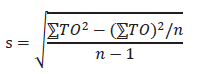
s = 13.80
Lastly, the number of observations is calculated as shown below:
N = (ts/TMk)2 = (2.2622 * 13.80 / 184.8 * 0.05)2
N = 11.415, then N = 12
Therefore, two additional observations must be added to the 10 preliminary selected, totaling 12 as shown in Table 1.
Model Formulation
Upon defining the problem and collecting data, the next step was to plan the model to represent the essence of the production process of the Manufacturing company. Shannon (1988) states that simulation is the process of developing a model of a real system, using past experience to understand its behavior or to evaluate new strategies while observing the restrictions imposed by a specific criterion or a set of standards for its proper functioning. Hence, the model under study focuses on the well-defined departments within the production process of the company. First, we observe the elaboration of the springs that make up the structure of the mattress, then we move to the machine that assembles the innerspring structure, then to the clinching area where the structure is reinforced, this is followed by quilting, closing and, finally, packaging.
Model Building
Real system models accurately represent the real world to be modeled. Model building is all about simplification. It is conducted to gain a better understanding of an aspect of the real world, as well as to explicitly clarify the meaning of complex relationships that exist in reality. According to García et al. (2006), ProModel focuses on the manufacturing processes of one or several assembly and manufacturing products, among others. Although minimal details of reality have been omitted, the model shows reality in all its aspects, allowing us to understand the existing complex relationships defined as exogenous and endogenous variables. Consequently, the results obtained in the research are valid.
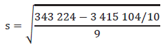
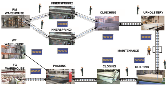
Figure 1 shows the company’s production system in the ProModel simulation program. The locations are the physical representation of the workstations where the entities that determine the production process arrive and leave. The locations included in the model are Innerspring, Clinching, Upholstery, Quilting, Closing, and Packing. The entities represent the overall product, that is, the mattress at the different manufacturing stages. For instance, we have springs, innerspring, reinforced innerspring, upholstered innerspring, quilted innerspring, closed mattress, and packed mattress. The arrivals of the entities determine their entry into the system; the simulation model starts with the arrival of the springs, as shown in Figure 1. Also, the model spans from the arrival of the spring at the raw material (RM) warehouse to the finished goods (FG) warehouse, where the finished mattresses arrive.
The processes are the set of operations that occur in the locations, channeling the times, resources, and other occurrences related to the entities. Variables are counters that helps us track the number of products being processed at a given moment in real time. For example, total number mattresses, rejected mattresses, structured mattresses, upholstered mattresses, quilted mattresses, closed mattresses, and packed mattresses. The resources are the workers that are part of the system, such as operator in charge of structuring, innerspring, upholstery, quilting, closing, and packing, as well as inspectors and technicians. According to the historical data for each location, the frequency distribution for each workstation that best represents the model to be simulated is determined, as shown in Table 3.
Table 3 Statistical Distribution of Processes of the Current Model.
| Number | Workstation | Distribution |
|---|---|---|
| 1 | Innerspring | Normal(347, 20.1) |
| 2 | Clinching | Normal(201, 17.3) |
| 3 | Upholstery | Normal(213, 15.6) |
| 4 | Quilting | Normal(217, 12.2) |
| 5 | Closing | Normal(185, 12) |
| 6 | Packing | Normal(133, 6.22) |
Source: Prepared by the authors.
Simulation Results
Based on the information gathered by means of techniques used in methods engineering, the results obtained for the respective analysis are presented. Similar to the conceptualization of the current model, the locations were taken as a starting point. The movement of the entities throughout the locations of the production process was also considered a principle. Table 4 shows the results of a run of the current simulation model expressed in seconds.
Table 4 Results of a Run of the Current Simulation Model.
| Name | Time (min.) | Capacity | Total Inputs | Average Time per Input | Average Content | Maximum Content | Current Content | Utilization (%) |
|---|---|---|---|---|---|---|---|---|
| RM Warehouse | 12 480.00 | 5000.00 | 1757.00 | 520.13 | 1.22 | 6.00 | 3.00 | 0.02 |
| Innerspring | 12 480.00 | 1.00 | 1753.00 | 349.82 | 0.82 | 1.00 | 0.00 | 81.90 |
| Clinching | 12 480.00 | 1.00 | 1753.00 | 197.67 | 0.46 | 1.00 | 0.00 | 46.28 |
| Upholstery | 12 480.00 | 1.00 | 1753.00 | 216.58 | 0.51 | 1.00 | 1.00 | 50.70 |
| Quilting | 12 480.00 | 1.00 | 1752.00 | 225.33 | 0.53 | 1.00 | 1.00 | 52.72 |
| Closing | 12 480.00 | 1.00 | 1751.00 | 187.47 | 0.44 | 1.00 | 0.00 | 43.84 |
| Packing | 12 480.00 | 1.00 | 1751.00 | 132.97 | 0.31 | 1.00 | 0.00 | 31.09 |
| FG Warehouse | 12 480.00 | 5000.00 | 1712.00 | 21.87 | 0.05 | 1.00 | 0.00 | 0.00 |
Source: Prepared by the authors.
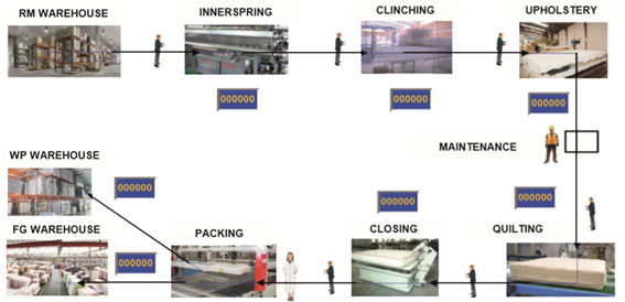
A comparison of the actual data and the data from the results obtained from the current model was made following the normal operation of the model (Table 7). Figure 2 shows the similarity of the data, thus indicating that the model is within the acceptance ranges, as verified using a Student’s t-test. First, data normal behavior is determined according to the following statistical hypothesis and decision rule:
Ho: The analyzed data have a normal behavior.
Ha: The analyzed data do not have a normal behavior.
Decision rules: If p ≥ 0.05, Ho is accepted.
If p < 0.05, Ha is rejected.
Table 5 Normality Test Results of Real Data and Simulation Data.
| Kolmogorov-Smirnova | Shapiro-Wilk | |||||
|---|---|---|---|---|---|---|
| Statistic | df | Sig. | Statistic | df | Sig. | |
| Real_Data | .328 | 6 | .043 | .863 | 6 | .201 |
| Promodel_Data | .295 | 6 | .113 | .885 | 6 | .294 |
a. Lilliefors Significance Correction.
Source: Prepared by the authors.
According to Table 5, p > 0.05 and Ha is accepted; therefore, data follow normal behavior. Subsequently, we conducted Student’s t-test considering the following statistical hypothesis and decision rule:
Ho. There is no significant difference between the means of the real and ProModel data.
Ha. There is a significant difference between the means of the real and ProModel data.
Decision rule: If p > 0.05, Ho is accepted.
If p ≤ 0.05, Ha is accepted.
Table 6 Student’s T-Test Results for Real Data and Simulation Data.
| Paired Samples Test | |||||||||
|---|---|---|---|---|---|---|---|---|---|
| Paired Differences | t | df | Sig. (2-tailed) | ||||||
| Mean | Std. Deviation | Std. Error Mean | 95% Confidence Interval of the Difference | ||||||
| Lower | Upper | ||||||||
| Par 1 | Real_Data- ProModel_Data | −2.83500 | 3.83489 | 1.56559 | −6.85947 | 1.18947 | −1.811 | 5 | .130 |
Source: Prepared by the authors.
From the results in Table 6, it is concluded that p > 0.05; therefore, Ha is accepted. There is no significance difference between the means of real data and ProModel data.
Table 7 Comparison of Real Data vs. Simulation Data.
| Workstation | Real Data (seconds) | ProModel Data (seconds) |
|---|---|---|
| Innerspring | 346.50 | 349.82 |
| Clinching | 200.33 | 197.67 |
| Upholstery | 212.50 | 216.58 |
| Quilting | 216.50 | 225.33 |
| Closing | 184.50 | 187.47 |
| Packing | 132.50 | 132.97 |
Source: Prepared by the authors.
The first 20 responses of the current model are taken from Table 8 for the calculation of the number of replications needed for the model as a pilot test. Based on the results to determine the sample size, 21 replications are necessary to statistically validate the model. First, it was necessary to determine this number of responses of the replicate using the classical method, according to the formula taken from Tamashiro and Yacarini (2018).
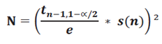
Where:
N : number of replications
n : sample size
𝒕 𝒏−𝟏,𝟏−∝/𝟐 : Critical value of Student’s t-distribution.
α : Significance level
s(n) : Standard deviation of the sample
e : Error between the population mean and the sample mean.
The following formula was used to determine the absolute error of the sample:
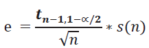
Based on these data, it was possible to analyze the behavior of the replications and determine the number of responses needed to validate the model. First, a sample mean of 1692.45 and a sample deviation of 4.978 were determined. This information made it possible to calculate the sampling error.
e = 2.093 * 4.978 / 20 = 2.33
Subsequently, the number of replications was calculated considering the sampling error value (2.33) at 95% confidence level.
𝑵= 𝟐.𝟎𝟗𝟑 𝟐.𝟑𝟑 ∗ 𝟒.𝟗𝟕𝟖 ² = 20.0008
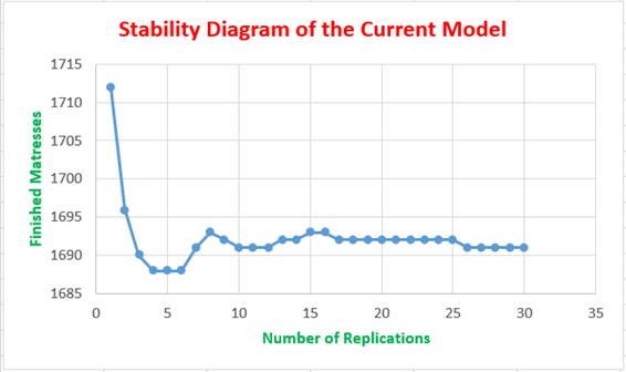
Using this result, we corroborated that 21 replications are sufficient to validate the current model simulation. For a more detailed analysis, Table 8 shows 30 replications of the current model, while Figure 3 shows the stability diagram of these replications, showing a fixed value trend.
Table 8 Result of the Replications of the Current Model.
| Replications | Available Time (hr) | Finished Mattresses | Rejected Mattresses | Mattresses per Hour |
|---|---|---|---|---|
| 1 | 208 | 1712 | 39 | 8.231 |
| 2 | 208 | 1696 | 44 | 8.154 |
| 3 | 208 | 1690 | 44 | 8.125 |
| 4 | 208 | 1688 | 43 | 8.115 |
| 5 | 208 | 1688 | 43 | 8.115 |
| 6 | 208 | 1688 | 42 | 8.115 |
| 7 | 208 | 1691 | 42 | 8.130 |
| 8 | 208 | 1693 | 42 | 8.139 |
| 9 | 208 | 1692 | 42 | 8.135 |
| 10 | 208 | 1691 | 42 | 8.130 |
| 11 | 208 | 1691 | 41 | 8.130 |
| 12 | 208 | 1691 | 41 | 8.130 |
| 13 | 208 | 1692 | 41 | 8.135 |
| 14 | 208 | 1692 | 42 | 8.135 |
| 15 | 208 | 1693 | 41 | 8.139 |
| 16 | 208 | 1693 | 41 | 8.139 |
| 17 | 208 | 1692 | 41 | 8.135 |
| 18 | 208 | 1692 | 42 | 8.135 |
| 19 | 208 | 1692 | 42 | 8.135 |
| 20 | 208 | 1692 | 42 | 8.135 |
| 21 | 208 | 1692 | 43 | 8.135 |
| 22 | 208 | 1692 | 43 | 8.135 |
| 23 | 208 | 1692 | 43 | 8.135 |
| 24 | 208 | 1692 | 43 | 8.135 |
| 25 | 208 | 1692 | 43 | 8.135 |
| 26 | 208 | 1691 | 44 | 8.130 |
| 27 | 208 | 1691 | 44 | 8.130 |
| 28 | 208 | 1691 | 44 | 8.130 |
| 29 | 208 | 1691 | 44 | 8.130 |
| 30 | 208 | 1691 | 44 | 8.130 |
Source: Prepared by the authors.
From the results, a bottleneck was detected in the innerspring area. Therefore, we decided to create a model by adding a new innerspring mattress machine to the production line, along with some other improvements shown in Table 9.
Table 9 Improvement Opportunities.
| Workstation | Current Situation | Improvement Opportunity |
|---|---|---|
| Innerspring | The operator has to inspect the springs to be used. | Springs come ready to be assembled. Idle time: 25 s. |
| Springs come out of the spring machine onto a side belt. | Springs have to be close to the workstation. Idle time: 9 s. | |
| Clinching | Innerspring structures are checked by the operator at the workstation. | Innerspring structures are reinforced and ready to be upholstered. Idle time: 22 s. |
| Innerspring structures are located in the work-in-process warehouse. | Innerspring structures have to be located close to the workstation. Idle time: 9 s. | |
| Upholstery | Innerspring structures are brought in from the work-in-process warehouse. | Innerspring structures have to be located close to the workstation. Idle time: 11s. |
| Upholstery comes in different sizes. | Upholstered panels have to match the exact size of the order. Idle time: 34 s. | |
| Quilting | Upholstered innerspring structures are brought in from the work-in-process warehouse. | Upholstered innerspring structures have to be close to the workstation. Idle time: 10 s. |
| Quilted material is oversized. | Foam has to be pre-cut to the exact size. Idle time: 36 s. | |
| Closing | Quilted innerspring structures are in the work-in-process warehouse. | All materials have to be close to the workstation. Idle time: 8 s. |
| Cover panel comes separated from the top and the seam is undone. | All materials have to be ready to be closed. Idle time: 12 s. | |
| Packing | Mattresses are brought in from the work-in-process warehouse. | Materials have to be close and ready to be packed. Idle time: 5 s. |
| Plastic is cut exceeding the size of the mattress. | Plastic have to be cut to exact measurements. Idle time: 15 s. |
Source: Prepared by the authors using the company’s data.
The principle of the improved model (Figure 4) was to move the entities throughout the locations. A new innerspring mattress machine was introduced to streamline the flow of the production line. All the improvements listed in Table 9 were also implemented, thus reducing the cycle times at the stations considerably. In addition, the transportation times in the current model were determined based on the distance from the workstation to the work-in-process warehouse. Distance times are already included in the cycle times of this model, where flow is continuous; however, an average time of 10 seconds is considered for picking up the product at the workstations and finishing the process. The normal distribution adapted to the proposed model was used, as shown in Table 10. The results of the improved model run are presented in Table 11.
Table 10 Statistical Distribution of the Improved Model.
| Number | Workstation | Distribution |
|---|---|---|
| 1 | Innerspring | Normal(322, 20.1) |
| 2 | Clinching | Normal(178, 16.6) |
| 3 | Upholstery | Normal(179, 15.6) |
| 4 | Quilting | Normal(181, 12.2) |
| 5 | Closing | Normal(173, 12) |
| 6 | Packing | Normal(118, 6.22) |
Source: Prepared by the authors.
Table 11 Simulation Results of the Improved Model.
| Name | Scheduled Time (min) | Capacity | Total Inputs | Average Time per Input | Average Content | Maximum Content | Current Content | Utilization (%) |
|---|---|---|---|---|---|---|---|---|
| RM Warehouse | 12 480.00 | 5000.00 | 3466.00 | 16.38 | 0.08 | 4.00 | 0.00 | 0.00 |
| Innerspring1 | 12 480.00 | 1.00 | 1726.00 | 328.09 | 0.76 | 1.00 | 1.00 | 75.63 |
| Innerspring2 | 12 480.00 | 1.00 | 1739.00 | 328.59 | 0.76 | 1.00 | 0.00 | 76.31 |
| Clinching | 12 480.00 | 1.00 | 3462.00 | 182.68 | 0.84 | 1.00 | 1.00 | 84.46 |
| Upholstery | 12 480.00 | 1.00 | 3460.00 | 187.48 | 0.87 | 1.00 | 1.00 | 86.63 |
| Quilting | 12 480.00 | 1.00 | 3458.00 | 182.12 | 0.84 | 1.00 | 1.00 | 84.10 |
| Closing | 12 480.00 | 1.00 | 3457.00 | 174.48 | 0.81 | 1.00 | 1.00 | 84.55 |
| Packing | 12 480.00 | 1.00 | 3456.00 | 118.05 | 0.54 | 1.00 | 1.00 | 54.49 |
| FG Warehouse | 12 480.00 | 5000.00 | 3373.00 | 10.00 | 0.05 | 1.00 | 0.00 | 0.00 |
Source: Prepared by the authors.
For the calculation of the number of replicates required for the improved model as a pilot test to determine the sample size, the first 20 responses of the runs are taken form Table 12. The number of responses of the replications was determined by the classical method, using the formula of the previous model. The absolute error of the sample was also determined using the same formula. These data made it possible to determine the number of responses needed to validate the model statistically. Also, the sample deviation was determined at 7.4544, allowing us to calculate the sampling error.
e = 2.093 * 7.4544 / 20 = 3.4887
Subsequently, the number of replications was calculated considering the sampling error value (3.4887) at 95% confidence level.
𝑵= 𝟐.𝟎𝟗𝟑 𝟑.𝟒𝟖𝟖𝟕 ∗ 𝟒.𝟗𝟕𝟖 ² = 20.0000
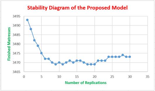
Using this result, we corroborated that 20 replications are sufficient to validate the current model simulation. For a more detailed analysis, Table 12 shows 30 replications of the improved model, while Figure 5 shows the stability diagram of these replications, showing a fixed value trend.
The model has a rather disorganized behavior at the beginning of the replications. The expected results then present a downward trend, but as the replications continue to increase, the model manages to stabilize at a fixed value.
Table 12 Results of the Replications of the Proposed Model.
| Replications | Available Time (hr) | Finished Mattresses | Rejected Mattresses | Mattresses per Hour |
|---|---|---|---|---|
| 1 | 208 | 3373 | 82 | 16.216 |
| 2 | 208 | 3398 | 81 | 16.337 |
| 3 | 208 | 3397 | 83 | 16.332 |
| 4 | 208 | 3396 | 83 | 16.327 |
| 5 | 208 | 3388 | 84 | 16.288 |
| 6 | 208 | 3386 | 87 | 16.279 |
| 7 | 208 | 3385 | 87 | 16.274 |
| 8 | 208 | 3383 | 89 | 16.264 |
| 9 | 208 | 3382 | 89 | 16.260 |
| 10 | 208 | 3380 | 91 | 16.250 |
| 11 | 208 | 3379 | 91 | 16.245 |
| 12 | 208 | 3380 | 91 | 16.250 |
| 13 | 208 | 3378 | 91 | 16.240 |
| 14 | 208 | 3375 | 91 | 16.226 |
| 15 | 208 | 3376 | 91 | 16.231 |
| 16 | 208 | 3376 | 90 | 16.231 |
| 17 | 208 | 3378 | 90 | 16.240 |
| 18 | 208 | 3377 | 91 | 16.236 |
| 19 | 208 | 3377 | 90 | 16.236 |
| 20 | 208 | 3378 | 90 | 16.240 |
| 21 | 208 | 3378 | 89 | 16.240 |
| 22 | 208 | 3378 | 90 | 16.240 |
| 23 | 208 | 3378 | 90 | 16.240 |
| 24 | 208 | 3379 | 90 | 16.245 |
| 25 | 208 | 3379 | 90 | 16.245 |
| 26 | 208 | 3379 | 90 | 16.245 |
| 27 | 208 | 3379 | 90 | 16.245 |
| 28 | 208 | 3379 | 89 | 16.245 |
| 29 | 208 | 3378 | 89 | 16.240 |
| 30 | 208 | 3379 | 89 | 16.245 |
Source: Prepared by the authors.
Gutiérrez (2010) states that productivity is related to the results obtained in a process or a system. Results for calculating productivity with the current method follow the formula below.
Productivity Index = Production/Resources
Productivity Ratio = 1712 mattresses/208 hours = 8.230 mattresses/hour
Productivity with the proposed method was calculated using the same formula as above, obtaining the results shown below.
Productivity Index = 3373 mattresses/208 hours = 16.216 mattresses/hour
From the results, a 97.02% increase in productivity is obtained using the proposed method.
A statistical analysis was performed to ratify the validity of the model. Table 13 shows 30 replications before improvements, and the same number for the proposed method for testing the hypothesis.
Table 13 Productivity Before and After Using the Simulation Model.
| Replications | Available Time (hr) | Before | After | ||
|---|---|---|---|---|---|
| Finished Mattresses | Mattresses per Hour | Finished Mattresses | Mattresses per Hour | ||
| 1 | 208 | 1712 | 8.231 | 3373 | 16.216 |
| 2 | 208 | 1696 | 8.154 | 3398 | 16.337 |
| 3 | 208 | 1690 | 8.125 | 3397 | 16.332 |
| 4 | 208 | 1688 | 8.115 | 3396 | 16.327 |
| 5 | 208 | 1688 | 8.115 | 3388 | 16.288 |
| 6 | 208 | 1688 | 8.115 | 3386 | 16.279 |
| 7 | 208 | 1691 | 8.130 | 3385 | 16.274 |
| 8 | 208 | 1693 | 8.139 | 3383 | 16.264 |
| 9 | 208 | 1692 | 8.135 | 3382 | 16.260 |
| 10 | 208 | 1691 | 8.130 | 3380 | 16.250 |
| 11 | 208 | 1691 | 8.130 | 3379 | 16.245 |
| 12 | 208 | 1691 | 8.130 | 3380 | 16.250 |
| 13 | 208 | 1692 | 8.135 | 3378 | 16.240 |
| 14 | 208 | 1692 | 8.135 | 3375 | 16.226 |
| 15 | 208 | 1693 | 8.139 | 3376 | 16.231 |
| 16 | 208 | 1693 | 8.139 | 3376 | 16.231 |
| 17 | 208 | 1692 | 8.135 | 3378 | 16.240 |
| 18 | 208 | 1692 | 8.135 | 3377 | 16.236 |
| 19 | 208 | 1692 | 8.135 | 3377 | 16.236 |
| 20 | 208 | 1692 | 8.135 | 3378 | 16.240 |
| 21 | 208 | 1692 | 8.135 | 3378 | 16.240 |
| 22 | 208 | 1692 | 8.135 | 3378 | 16.240 |
| 23 | 208 | 1692 | 8.135 | 3378 | 16.240 |
| 24 | 208 | 1692 | 8.135 | 3379 | 16.245 |
| 25 | 208 | 1692 | 8.135 | 3379 | 16.245 |
| 26 | 208 | 1691 | 8.130 | 3379 | 16.245 |
| 27 | 208 | 1691 | 8.130 | 3379 | 16.245 |
| 28 | 208 | 1691 | 8.130 | 3379 | 16.245 |
| 29 | 208 | 1691 | 8.130 | 3378 | 16.240 |
| 30 | 208 | 1691 | 8.130 | 3379 | 16.245 |
Source: Prepared by the authors.
Using the data in Table 13, the normality test is performed, considering the following statistical hypothesis and decision rule.
Ho: The analyzed data have a normal behavior
Ha: The analyzed data do not have a normal behavior.
Decision rule: If p > 0.05, Ho is accepted. If p ≤ 0.05, Ha is accepted.
Table 14 Normality Test Result.
| Kolmogorov-Smirnova | Shapiro-Wilk | |||||
|---|---|---|---|---|---|---|
| Statistic | df | Sig. | Statistic | df | Sig. | |
| Productivity_Methods_Before | .360 | 30 | .000 | .501 | 30 | .000 |
| Productivity_Methods_After | .291 | 30 | .000 | .756 | 30 | .000 |
Lilliefors Significance Correction.
Source: Prepared by the authors.
From the results in Table 14, p < 0.05, and the null hypothesis (Ho) is rejected; therefore, the data do not have a normal behavior. Consequently, a non-parametric statistic test must be used for hypothesis testing; the Wilcoxon test was chosen. Statistical hypothesis and decision rule for this case are presented below.
Ho. The implementation of methods engineering does not improve the productivity of the production process of a manufacturing company.
Ha. The implementation of methods engineering does improve the productivity of the production process of a manufacturing company.
Decision rule: If p > 0.05, Ho is accepted. If p ≤ 0.05, Ha is accepted.
Table 15 Descriptive Statistics of Productivity Considering Methods Engineering Improvements.
| Descriptives | |||||
|---|---|---|---|---|---|
| Mean | Median | Deviation | Minimum | Maximum | |
| Productivity_Methods_Before | 8.13540 | 8.13500 | .019604 | 8.115 | 8.231 |
| Productivity_Methods_After | 16.25440 | 16.24500 | .030240 | 16.216 | 16.337 |
Source: Prepared by the authors.
In Table 15, it is observed that the comparison between the mean and median of productivity before is lower than the mean and median of productivity after. However, the decision rule states that when p-value is less than or equal to 0.05, the Ho is rejected and Ha is accepted. The Wilcoxon test statistic can be used to support this result.
Table 16 Wilcoxon Test Statistics Considering Methods Engineering Improvements.
| Test Statisticsa | |
|---|---|
| Productivity_Methods_After - Productivity_Methods_Before | |
| Z | −4.790b |
| Asymp. Sig. (2-tailed) | .000 |
a. Wilcoxon Signed Ranks Test.
b. Based on negative ranks.
Source: Prepared by the authors.
From the results in Table 16, it is concluded that p < 0.05; therefore, the null hypothesis (Ho) is rejected. This means that the samples correspond to different populations. In this case, the second sample corresponds to an improvement in production through the application of methods engineering. The application of method engineering improves the productivity of the production process of a manufacturing company.
DISCUSSION
A great similarity in the comparison of results was observed during the validation of the methods engineering model. As there is no significant difference between the means of the real data of the simulation results, the approach and the representation of reality are within acceptable ranges. These results are supported by the statistical analysis made for the comparison of ranges between “productivity before” and “productivity after”. It was demonstrated that the samples come from different populations and that the second one corresponds to an improvement in production through the application of methods engineering techniques, achieving an improvement of up to 97.02% of productivity increase. These results are consistent with those of Arnold and Osorio (1998), who state that system models are presented as a systematic and scientific way of approaching and representing reality. Furthermore, the results on productivity increase coincide with those obtained by Jiménez and Gómez (2014), who implemented a model to evaluate and recommend improvements in a human consumption food distribution center and obtained a system performance increase of approximately 40%.
CONCLUSIONS
It is evident from the results obtained that the application of a discrete simulation model can improve the productivity of the production process of the manufacturing company under study by 97.02%.
A comparison of the operation times of the observed data and the data obtained from the simulation program shows great similarity. A statistical test verifies that there is no significant difference between the means of the observed data and the data provided by ProModel; therefore, the results adequately represent the company’s production process.
In order to validate the proposed simulation model of the company’s production process, it was necessary to study the behavior of the replicates. It was determined that 20 replicates are sufficient to validate the model.
REFERENCIAS
Arnold, M., y Osorio, F. (1998). Introducción a los conceptos básicos de la Teoría General de Sistemas. Cinta Moebio. Revista de Epistemología de Ciencias Sociales, (3), 40-49. [ Links ]
Behar Rivero, D. S. (2008). Metodología de la investigación. Praia, Cabo Verde: Shalom. [ Links ]
Cevallos Carrillos, J. A., Fernández Ledesmo, J. D., y Restrepo Núñez, E. D. (2013). Aplicación de un modelo de simulación discreta en el sector del servicio automotor. Revista Ingeniería Industrial, 1(1), 51-61. https://repository.upb.edu.co/handle/20.500.11912/6489 [ Links ]
Fishman, G. S. (1978). Conceptos y Métodos en la simulación de eventos discretos. México: Limusa Wiley. [ Links ]
Forero-Páez, Y., y Giraldo, J. A. (2016). Simulación de un Proceso de Fabricación de Bicicletas. Aplicación Didáctica en la Enseñanza de la Ingeniería Industrial. Formación Universitaria, 9(3), 39-50. [ Links ]
García Dunna, E., García Reyes, H., y Cárdenas Barrón, L. E. (2006). Simulación y Análisis de Sistemas con Promodel. Naucalpán de Juárez, México: Pearson Educación. [ Links ]
Gutiérrez Pulido, H. (2010). Calidad total y Productividad. México D. F., México: McGraw-Hill. [ Links ]
Hernández Sampieri, R., Fernández Collado, C., y Baptista Lucio, P. (2014). Metodología de la Investigación. México D.F., México: McGraw Hill. [ Links ]
Iglesias León, M., y Cortés Cortés, M. E. (2004). Generalidades sobre Metodología de la Investigación. Campeche, México: Universidad Autónoma del Carmen. [ Links ]
Jiménez, M., y Gómez, E. (2014). Mejoras en un centro de distribución mediante la simulación de eventos discretos. Industrial Data. 17(2), 143-148. [ Links ]
Sellie, C. N. (2006). Estudios de tiempos con cronómetro. En Maynard, M., y Hodson, W. (Eds.), Manual del Ingeniero Industrial (pp. 4.13-4.38). México D. F., México: McGraw Hill. [ Links ]
Merino, A., Acebes, L. F., Mazaeda, R., y De Prada, C. (2009). Modelado y Simulación del Proceso de Producción del Azúcar. Revista Iberoamericana de Automática e Informática Industrial (RIAI), 6(3), 21-31. [ Links ]
Naylor, T., Balintfi, J., Burdick, D., y Chu, K. (1991). Técnicas de simulacion en computadoras. México D. F., México: Limusa. [ Links ]
Niebel, B. W., y Freivalds, A. (2009). Ingenieria Industrial. Métodos, Estándares y Diseño del Trabajo. México D. F., México: McGraw Hill . [ Links ]
Palacios Acero, L. C. (2016). Ingenieria de Métodos. Movimientos y Tiempos. Bogotá, Colombia: ECOE Ediciones. [ Links ]
Shannon, R. E. (1988). Simulación de Sistemas. Ciudad de México, México: Trillas. [ Links ]
Tamashiro Tamashiro, E., y Yacarini Vadillo, C. J. (2018). Propuesta de mejora de la productividad mediante la aplicación de la metodologia de Manufactura Esbelta en el área de producción de una fábrica de calzados para damas. (Tesis de grado). Universidad Peruana de Ciencias Aplicadas, Lima. [ Links ]
Received: October 03, 2022; Accepted: March 03, 2023
 Este es un artículo publicado en acceso abierto bajo una licencia Creative Commons
