


Servicios Personalizados
Revista

Articulo
 Inglés (pdf)
 Articulo en XML
 Referencias del artículo
 Enviar articulo por email
Indicadores
-
 Citado por SciELO
Links relacionados
-
 Similares en
SciELO
Similares en
SciELO
Compartir

 Permalink
Journal of Economics, Finance and Administrative Science
versión impresa ISSN 2077-1886
Journal of Economics, Finance and Administrative Science v.16 n.31 Lima dic. 2011
ARTICLES
Linkages between Value based Performance Measurements and risk return trade off: theory and evidence*
Vínculos entre las mediciones de valor basado en el desempeño y el dilema riesgo retorno: teoría y evidencia
Saban Celik1 ; Banu Esra Aslanertik2
* The authors thank Ali M. Kutan (editor); Robbie Brada (Managing Director) and conference participants in The Society for the Study of Emerging Markets EuroConference 2010 and 5th International Conference on Business, Economics and Management, Izmir, Turkey, 22-24 October 2009.
1 Financial Consultant and instructor, Deparment of International Trade and Finance, Yasar University, Universite Street, Izmir. <saban. celik@yasar.edu.tr>.
2 Associate Professor, Department of Accounting and Finance, Dokuz Eylul University, Kaynaklar Campus, Izmir, Turkey. <esra. aslanertik@deu.edu.tr>.
Abstract
In this study we attempt to investigate the linkages between value-based performance measurements and risk-return trade off in a way to explain cross sectional asset returns. On the side of value based performance measurements, three groups of variables are used as a sorting factor: traditional measures which consist of accounting based and market based; recently popularized measures such as Economic Value Added and Market Value Added and theoretically sound measures such as foreign investor allocation and firm systematic risk indicators. The goals of the study are (i) to show how value based measurements techniques relate to risk return trade off and (ii) how these measures affect the cross sectional asset returns in manufacturing industry. Empirical results indicate that foreign investor allocation as a sorting factor produces much more meaningful risk return positive linear relation for cross sectional asset returns than traditional and recently popularized measures.
Keywords: Asset pricing, risk, Value Added Measures, emerging markets.
Resumen
En este estudio se intenta investigar los vínculos entre las mediciones de valor basado en el desempeño y el dilema de riesgo retorno para explicar los retornos de valores diversificados. Por el lado de las mediciones de rendimiento sobre el valor se utilizaron tres grupos de variables como factor de clasificación: mediciones tradiciones, que consisten en mediciones de contabilidad y de mercado; otras mediciones recientemente popularizadas como el Valor Económico Añadido (VEA), el Valor de Mercado Añadido (VMA) y mediciones teóricamente sólidas como la asignación de la inversión extranjera e indicadores estables sistemáticos de riesgo. Los objetivos de este estudio son: (i) demostrar cómo las técnicas basadas en mediciones se relacionan con el riesgo de retorno de compensación, y (ii) cómo estas mediciones afectan los retornos de valores diversificados en la industria manufacturera. Estudios empíricos indican que la asignación de inversión extranjera como un factor de clasificación produce mucho más riesgo significativo de relación linear positiva para el retorno de valores diversificados que las mediciones tradicionales y las de reciente popularización.
Palabras claves: Riesgo de fijación de precio de valores, Mediciones de Valor Añadido, mercados emergentes.
INTRODUCTION
The primary objective of this paper is to examine one of the core concepts of finance, asset pricing, for the purpose of explaining asset dynamics which have been extensively analyzed by economists, statistician, econometrician, mathematician and financial scholars. More interestingly asset pricing becomes a starting and also pioneering area for many groundbreaking models and extents new perspectives in several fields. In the simplified term, asset pricing can be defined as a common field of economics, finance, mathematics, statistics, econometrics and even psychology. In order to emphasize why study asset pricing, Cochrane (2005) underlined that:
Asset pricing theory tries to understand the prices or values of claims to uncertain payments. A low price implies a high rate of return, so one can also think of the theory as explaining why some assets pay higher average returns than others. To value an asset, we have to account for the delay and for the risk of its payments. The effects of time are not too difficult to work out. However, corrections for risk are much more important determinants of many assets values. For example, over the last 50 years U.S. stocks have given a real return of about 9% on average. Of this, only about 1% is due to interest rates; the remaining 8% is a premium1 earned for holding risk. Uncertainty or corrections for risk make asset pricing interesting and challenging (xiii).
The challenging point as Cochrane underlined is coming from how to adjust the risk under uncertainty. The way we approach the problem is a rather naive way of thinking which can be seen as a common way of financial economists as follows2: We would like to start with the following question: Is price3 of an asset equal to its value4?
Such a simple question can be easily answered as "No". However, this seemingly simple question can lead us thinking of under which conditions such equality will be held. It is often heard that "this car is sold below its value" or "the firm asset is lower than its market price". It seems that the price and the value are two different concepts. On the one hand, there is an indicator that is price and on the other hand, there is a notion, value, which is quantified through a price. However, the main difference is the factors that affect price and value. This paper is the first attempt to examine the linkages between risk-return trade off based on value based performance measurements. The second section shows theoretical roots of asset value and pricing process. In the third section, we review the literature devoted to value based performance measurements and in section four we offer empirical analyzes of the linkages between value based performance measurements and risk-return trade off.
THEORETICAL LINKAGES BETWEEN VALUATION AND PRICING
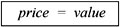
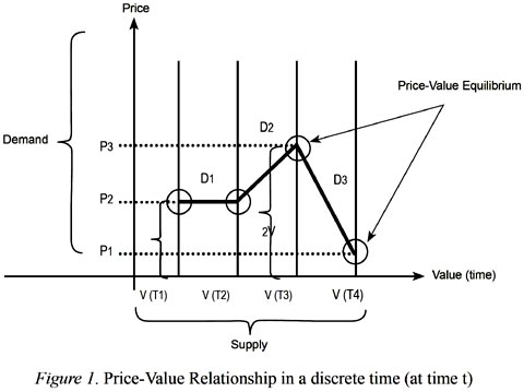
Figure 1 describes the price-value relationship whereas it is far away from being realistic representations. The main purpose is to draw a general framework to show how equilibrium exists under the factors that affect price-value equilibrium5 level. The main factor that affects the price of an asset is its demand in market. If there is no demand for a particular asset, it does not make any sense to price it. It is implicitly assumed that such asset can be marketable. On the other spectrum, the main factor that affects the value of the asset is its supply side. A car producing firm does not sell all of its products on the same price. "Why?" Since the qualifications of cars are different, their prices are quoted on different levels.
In a formal demonstration, we define the following properties:
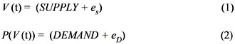
where V(t) is value function with respect to time (t), SUPPLY is the main factor (but only) affecting the value creation process; eis undefined factor affecting the process; P(V(t)) is price function with respect to value function V(t); DEMAND is the main factor (but only) affecting the price; eD is undefined factor affecting the process.
Proposition 1: the value of the asset is constant at certain time, t.
Proof 1: if we stop time, the value of any asset, including human value, will be fixed. As human beings, we would not turn older since time has been stopped.
Proposition 2: if we hold the demand constant between the two periods, the price of the asset will not be changed unless the value of the asset is changed.
Proof 2: What makes the value of any asset different in the public is its desirability, its demand. We implicitly assumed that the covariance between supply and demand is zero. However, it is true that supply and demand affect each other. The critical justification here that saved and proved our proposition is to isolate the impact of demand on supply and therefore on value, as depicted in Figure 1.
It is not intended to say that the demand and the supply do not affect each other and price-value equilibrium. This is a general framework in the sense that the price-value equilibrium is nothing more than a theoretical discussion. However, the definitions we used for value and price play important role behind the above discussion. We emphasize the role of value and assume that there exists a value before demand which determines its price level. The critical task is to establish its real (actual) value (equivalently economists used the term fair value and accountants used the term intrinsic value). The present paper does not claim that there are no other factors affecting the value and price or equivalently supply and demand for a given asset.
For this reason, we define eand eD as an undefined component of our theoretical discussion. The unique part of this view is that we do not follow utility based equilibrium as it is classical in determining prices in economics. We emphasize a more compact form and derive the theoretical linkages between value and price. In a discrete time setting, we showed how equilibrium existed in Figure 1. It is necessary to describe what kind of process there should be for price and value in continuous time (intertemporal settings).
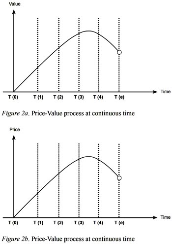
In Figures 2a and 2b, a representative value process is depicted. As it is seen, this representativeness looks like a product life cycle (or equivalently life cycle of the firm). It can not be extended for all products because some products such as consol, a financial product paying fixed cash payments developed and maintained by Bank of England Consols, simply have no maturity. However, in Figures 2a and 2b there is an ending time, T (e), for the product. The important inference derived from them is that at equilibrium, the (ending) price and the (real) value for the asset is the same. In other words, at time t (1), the value of the asset is a vertical line implying that there is a constant value for the asset. The level of its price is determined by its demand at time t (1) and the corresponding point represents the equilibrium price-value point. However, it is simply assumed that the demand for the asset depending upon the value of the asset may change, so that the level of the price in-creases or decreases. At the ending period, since there is no value for the asset at all, it should not be expected to be priced, as indicated by an empty circle in Figures 2a and 2b. The most difficult part in the described framework is how to define the exact price and value process for different assets, such as financial assets or nonfinancial assets or even for human capital.
Economists usually make specified assumptions to clarify the situation in which their predictions will be held. Let us start with a general case to emphasize how a value of an asset can be determined in one period model.
-
Assumption 1
Assumption 2: There is zero interest rate.
Assumption 3: There is zero inflation.
Assumption 4
Assumption 5: The rest of the factors that may affect the transaction remains constant at two dates (ceteris paribus). This assumption is required for the existence of price-value equilibrium. As it is noted earlier, if we hold the demand constant between the two periods, the price of the asset will not be changed unless the value of the asset is changed.
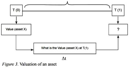
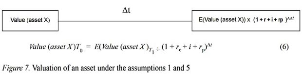
Figures 3 to 7 show how a value of an asset can be changed under these assumptions and in lack of assumptions 2, 3 and 4 mentioned above.
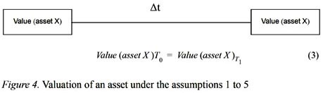
Under the assumptions 1 to 5, it is clear that we are certainly dealing with a sure value due to the fact that we fixed every factor that may affect the value of an asset in one way or another in the next period. This is the starting point to illustrate from certain to uncertain value. Despite the fact that valuation under uncertainty is the main theme of asset pricing, in this section we will just present it in a simplified manner.
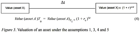
Relaxing assumption 2: There is a constant interest rate that can be earned in the market (later we will define this rate as risk free).
Introducing a constant interest rate leads us to discount the next period value to the present. As it is well documented in financial text books, present value calculation is usually used to evaluate the required rate of project. How this rate is to be determined is the subject of the models that are explained in the following sections.
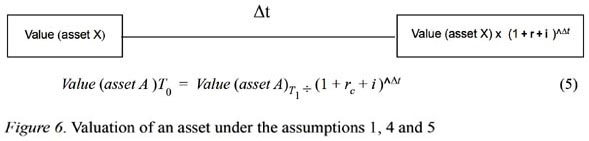
Relaxing assumption 2 and 3: There is a constant interest rate denoted as rthat can be earned in the market and an inflation rate, denoted as i (inflation is usually assumed that it is adjusted in risk free rate or in risk premium whereas it is necessary to demonstrate how it takes place in valuation).
The value of a Turkish Lira today is not equal to the value of a Turkish Lira tomorrow if there is an inflation and equivalently opportunity cost. The impact of inflation results on nominal returns and we usually deduct the impact and gain the real return. Therefore, the inflation rate may be added to constant rate to discount the next period value to the present.
Relaxing assumption 2, 3, and 4: There is a constant interest rate denoted as rthat can be earned in the market, an inflation rate, denoted as i and the risk that gives a premium denoted as rp (risk premium is a rate that is required for investors to take on; otherwise, the question is why investors invest if there is a certain rate that can be earned without taking any risk). Since there is an uncertainty, we will expect what will be the value of asset X at time T(1).
The fundamental relation between risk and return is assumed to be linear, at least at a theoretical point of view. In addition, it is also assumed that investors should be compensated for bearing the risk. This is called premium for bearing the risk. We assumed that the rate for bearing risk is a certain rate on the contrary to adjusting it for investors behaviors or market structure. This is overly simplifying the problem, whereas it is useful to demonstrate it and compare the result with what Capital Asset Pricing Model (CAPM) suggests.
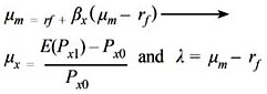
If we rearrange the expression (6) asV(asset X )T0 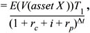 and since this is one period model Δt is set to 1 and we assume that inflation is inherit in risk premium or in constant interest rate in addition to defining constant interest rate as risk free and risk premium as βx excess market return. Hence, we would have the celebrated Sharpe-Lintner Capital Asset Pricing Model or CAPM (Sharpe, 1964; Lintner, 1965). CAPM states that expected return (μx) of an asset is equal to risk free rate (rf) plus assets risk premium (βx(μm – rf)) (μm is denoted hypothetical market portfolio return which consists of all assets).

Let us rearrange the CAPM in terms of returns:
Then, after the relevant adjustment we will have the following equation:
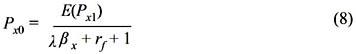
We can see that expressions (6) and (8) are quite similar even though their theoretical backgrounds are not identical. The difference in both equations is what constitutes denominator in discount factor and the way we approach the equilibrium.
VALUE PERFORMANCE MEASUREMENTS
In todays market most of the companies have recognized the importance of performance measurement within a broader view. Many researches have been made to emprically derive the importance of performance measurement in order to achieve financial excellence. The current financial environment, which can be characterized by new challenges, forced companies to develop value based performance measures to tackle the inefficiencies of traditional performance measures.
Value Based Management (VBM) is considered as a framework or management approach that aims to create long-term value for shareholders by producing returns in excess of the cost of capital, satisfying product markets and making measurement based on share price performance and dividend growth (Marsh, 1999; Ronte, 1998; Simms, 2001).Another definition made byArnold (1998) focuses on process view of VBM and defines it as a managerial approach focusing on shareholder wealth maximization through the guiding of its systems, strategies, processes, techniques, performance measurements and culture. The maximization of shareholder value directs company strategy, structure and processes.
In many different studies, it was stated that accounting based performance measures, such as net profit, return on investment and return on equity, are inadequate measures of financial performance especially in evaluating the goal of achieving value creation for shareholders (Rappaport 1986; Biddle, Bowen, & Wallace, 1997). Besides various definitions of VBM, by giving the benefits of it, we can clearly demonstrate that it helps to better deal with increased complexity, greater uncertainty and risk. Measuring for value and performance is a very powerful mangement tool; but it has a disadvantage: it requires too much detail or use metrics that are over-complex. Extreme caution must be made not to measure the wrong items as this may almost certainly lead to value destruction (Aslanertik, 2007).
Accounting based performance measures focus on the past: transactions-oriented, highly dependent on the choice of measurement method, conservatively biased, ignore some economic values and value changes that accountants feel cannot be measured accurately and objectively, ignore the cost of equity capital, ignore risk and changes in risk (Merchant & Sandino, 2009). Conversely, value based measures are both future and risk oriented while capturing real value creation. According to many people in Europe, and to a lesser degree in North America, VBM relates to deployment of the logic of Economic Value Added (EVA), Shareholder Value Added (SVA) or Market ValueAdded(MVA). Allofthesedeterminetherelative value of earnings to the cost of money. In each case, SVA,MVAandEVAare measurements.Inotherwords, when defined this way, VBM is about the focusing of managersenergy to applyorganization efforts towards maximizing financial performance.
The most popular value-based performance measure is Stern Stewarts Economic ValueAdded (EVA). EVAis the financial performance measure that most accurately reflects a corporations true profit (Stewart, 1991). This measurement is the difference between a companys net operating income after taxes and its cost of capital of both equity and debt (Stewart, 1994). EVAaccepts the assumption that the primary financial objective of any business is to maximize the wealth of its shareholders. Returns over and above the cost of capital increase shareholder wealth, while returns below the cost of capital erode shareholder wealth. Both academics and practitioners point out numerous benefits of EVA. Because it is a single period measure, it allows for an annual measurement of actual not-estimated or forecasted, value created performance (Armitage & Fog, 1996 ) Others refer to the fact that it corresponds more closely to economic profit than accounting earnings do and, as an objective, is consistent with the pursuit of shareholder interest.
Shareholder value added ( SVA ) is defined as the difference between the present value of incremental cash flow before new investment and the present value of investment in fixed and working capital.
SVA = (Present value of cash flow from operations during the forecast period + residual value + marketable securities) – Debt
Rappaport (1998) coined SVAto refer to the increase in shareholder value over time. Rappaport developed a shareholder value network which depicts the essential link between the corporate objective of creating shareholder value and the basic valuation or value drivers.The value driver model is a comprehensive approach that centers on seven key drivers of shareholder value, i.e. sales growth rate, operating profit magrin, income tax rate, working capital investment, fixed capital investment, cost of capital and forecast duration.
Market value added (MVA) is the difference between the equity market valuation of a company and the sum of the adjusted book value of debt and equity invested in the company.
MVA = market value – invested capital
This is a measure of the value generated by managers for shareholders. It captures both valuation – the degree of wealth enrichment for the shareholders and performance (i.e. the market assessment of how effectively a firms managers have used the scarce resources under their control ) – as well as how effectively management has positioned the company on the long term (Ehrbar, 1998).
MVA is said to be a more effective investment tool than other measures such as market value of equity, book/price ratio and price/earnings ratio (Yook & McCabe, 2001). Some empirical studies in literature supports the idea that EVA is superior to all other traditional accounting measures (Grant,1996; Lehn & Makhija, 1997; OByrne, 1996; Uyemura, Kantor, & Pettit,1996; Walbert, 1994), while some others proved the opposite (Biddle et al., 1997; Chen & Dodd, 2001; Clinton & Chen, 1998; Ray, 2001). Grant (1996) focused on the MVA/CAPITAL and EVA/CAPITAL ratios to adjust for firm size. The study concludes that EVA has a significant impact on the market-value-added of a firm and this wealth effect stems from the companys positive residual return on capital.
In addition, some studies investigated the relationship of different performance measures to stock price and stock returns (Clinton & Chen 1998; Chen & Dodd 2001 ). They observed that EVA was the only measure that did not significantly related to either stock price or stock return. Their findings also did not support the idea that EVA is the best measure for valuation purposes.
Bacidore et al. (1997) defined another performance measure, a refinement of EVA, and examined its statistical properties. This performance measure is called as Refined Economic Value Added (REVA). It complements EVA in a way that it could be used in conjunction with EVA, with the choice of measure dictated by the level of the organization at which the performance measure is used. They argued that REVA is a better measure of performance for top management, although EVA may be useful at lower levels. They computed REVA for a given period t is defined as follows:
REVAt = NOPATt - kw(MVti),
where NOPATt is the firms NOPAT at the end of period t, and MVt-i is the total market value of the firms assets at the end of period t -1 (beginning of period t). MVt-1 is given by the market value of the firms equity plus the book value of the firms total debt less non-interest-bearing current liabilities, all at the end of period t -1.
Modigliani and Miller (1963) established that the value of a company depends on three elements: the unleveraged value of the company, the value of the tax shields resulting from the existing debt, and the negative value created by the potential bankruptcy costs. Depending on this and EVA logic, Xavier and Pere (2003) proposed a corporate valuation formula that consistently reconciles the different value drivers contained in the traditional valuation models which was called Financial and Economic Value Added (FEVA). They have mathematically demonstrated that FEVA is related to the traditional Discounted Cash Flow (DCF) models.
Within the literature review above, in order to achieve higher performance and to become as successful as possible, companies may apply different measures or use various approaches for a variety of cases or problems. But it is obvious that each of these measures have some advantages and disadvantages or some shortcomings. Also, it is difficult to identify one single approach or measurement that will satisfy the need to all relevant problems, issues or cases. So, there can be several alternatives available in order to be successful. Considering all, the aim should be performing an integrated approach and simultaneous usage of different measures.
RESEARCH METHODOLOGY
Research methodology developed here has two main objectives: (i) to investigate the role of traditional value measures, recently popularized value measures and the two theoretically sound factors (stock betas and total foreign allocation in these stocks) with the risk return trade-off; and (ii) to examine the linkages between value measures and performance measures.
The empirical investigation conducted on two main pillars of finance-risk return trade off and portfolio performance is the first attempt to link and examine the soundness of accounting and market based measures to the theoretically generalized implications. While testing linearity, Celik et.al. (2009) analyzed the impact of Foreign Total Investor Allocation as a sorting procedure on risk-return trade off and reported highly significant relation based on monthly data6.
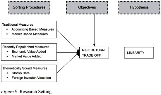
Table 1 demostrates the measures and their identity. Formulation for portfolio performance measures can be explained as follows: Sharpes measure divides average portfolio excess return over the sample period by the standard deviation of returns over that period. Like Sharpes, Treynors measure gives excess return per unit of risk, but it uses systematic risk instead of total risk. Jensens measure is the average return on the portfolio over and above that predicted by the S-L CAPM, given the portfolios beta and the average market return. The appraisal ratio divides the alpha of the portfolio by the nonsystematic risk of the portfolio. It measures abnormal return per unit of risk that in principle could be diversified away by holding a market index portfolio.
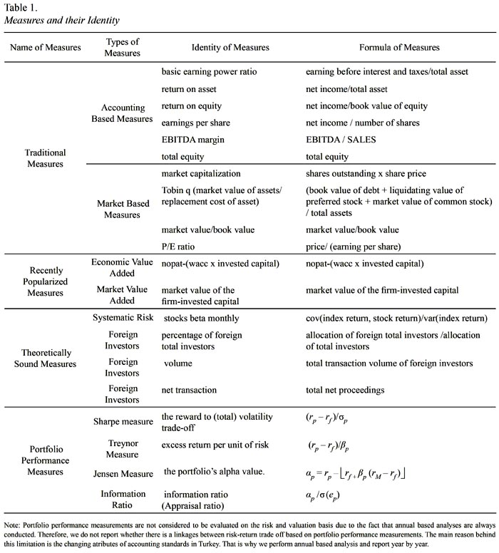
Tobins q is often used as a measure of the real value created by a firms management. The higher the q, the more value is added. The estimation of the replacement cost of assets is fairly difficult. One approximation was proposed by Lindenberg and Ross (1981). In this approximation, the numerator is the sum of the book value of debt (adjusted for age), market value of common equity, and book value of preferred stock, less net short-term assets. The denominator is total assets plus an adjustment for inflation on the firms equity capital. These calculations can be quite complex with respect to the debt adjustment and the inflation adjustment.
The proxy we used has been shown to be empirically close to the more complex Lindenberg and Ross proxy (Chung & Pruitt 1994; Perfect & Wiles 1994;Peterson & Peterson, 1996). For example, Perfect and Wiles compare five different proxies, ranging from the very complex to the simplest, and find that these proxies differ somewhat when comparing q-values for firms but are not substmtially different when looking at changes in q-values.
HYPOTHESES DEVELOPMENT
In the context of the paper, we classify three main streams of hypotheses: Hypotheses regarding to test linearity under the objective of risk-return trade off (i) when sorting factor is a traditional measures; (ii) when sorting factor is a recently popularized measure; and, (iii) when sorting factor is a theoretically sound measure. In a formal way, these hypotheses can be constructed as follows:
-
H1: There is positive linear relationship between realized mean return and risk when stocks sorted based on traditional measures (accounting and market based);
-
H2: There is positive linear relationship between realized mean return and risk when stocks sorted based on recently popularized measures;
-
H3: There is positive linear relationship between realized mean return and risk when stocks sorted based on theoretically sound measures.
Raw Data Transformation and Empirical Model
Monthly adjusted returns of common stocks are computed as follow (ISE, 2008):
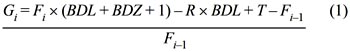
where Gi : return of month i; Fi : closing price of month i; BDL : number of stocks bought from using right issues during the month ; BDZ: number of stocks bought from using bonus issues during the month; R : price of pre-emptive rights ; T : dividend distributed per 1000 TL/1 YTL nominal value of one share ; Fi-1 : closing price of month i-1.
ISE National 100 Index is determined as a proxy of market portfolio and The Central Bank O/N interest rate is determined as a proxy of risk-free rate. ISE National 100 index is the only index that is being computed since the establishment of ISE, and hence, the most appropriate one representing the market portfolio. It is a type of weighted average index and is computed as follow:
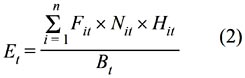
where Et: index value at time t ; n : number of stocks in the index (which is 100) ; Fit : price of stock i at time t ; Nit : total number of issued stocks of I ; Hit : ratio of public offering of stock i at time t ; Bt : adjusted-base market cap.
Using the market model regression for each asset, the following regression model employed so-called first-pass regression7:

where the term E(Rit) is stock i return at time t; Rf is risk free rate; E(RMt) is index return used as proxy for market portfolio; αi and βi are the estimated parameters of the model and they represent expected abnormal return and systematic risk level respectively. εit indicates white-noise error term which has zero mean and constant variance. In addition to that, covariance between the term εit and market risk premium denoted by E(RMt) – Rf is equal to zero which means that error term of the model is independent of market risk premium.
Cross-sectional Investigations (2002:01-2008:06 )
Linearity between risk and return is a long standing debate in financial literature. Fundamentally true relationship between risk and return is that there is high risk for high return or vise versa. The neo-classical financial model that explains this relation is S-L CAPM among its variants. S-L CAPM states that expected return (µ) of an asset is equal to risk free rate (rf ), plus assets risk premium (βx (µm– rf)). (µis denoted hypothetical market portfolio return which consists of all assets).

In financial literature, S-L CAPM is tested in form of equation (3) so that we derive beta coefficient from first pass regression and obtain an indicator for risk. Second step is to calculate average mean return of stocks analyzed here. Estimating Security Market Line is a cross sectional regression procedure in testing linearity of risk and return so called second pass regression. Previously, we employed regression in equation (3) for every single stocks analyzed; then, calculate sample averages of the excess return on each of the stocks from the full sample,  , sample estimates of beta coefficients o each of the stocks, βi , sample average of the excess return of the market index,
  and following regression is conducted:
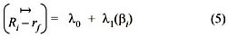
where:
λ
0 and λ1 are coefficients of regressions that should be tested against λ0 = 0 and λ1 = The economic meaning of alpha term in equation (5) is that there is zero expected abnormal return in equilibrium. Beta term, on the other hand implies that risk premium should be equal to risk premium of the market portfolio. However, we simply cannot observe hypothetical market portfolio so that we use a proxy index return for it. In most cases, the highest index in terms of market capitalization is used as it is the case here (ISE 100 Index is used here). We calculate real risk free rate over Central Bank over night interest rate with Consumer Price Index within the same time period and get 0.94 average monthly excess return, which is economically tested against regression beta coefficient of (5) (Tables 2 and 3).
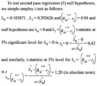
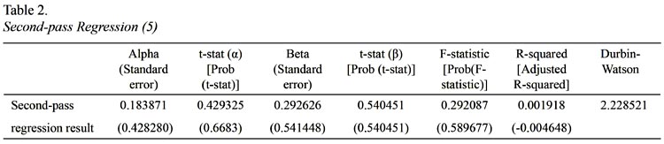
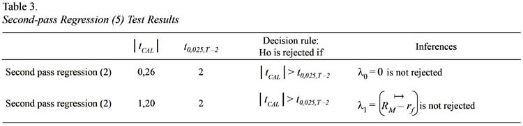
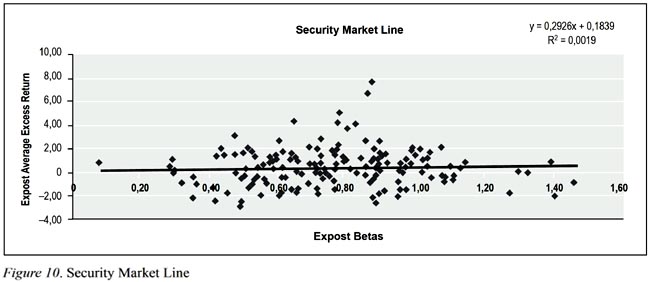
Second pass regression (5) results do not support well the linear relationship between average excess return which is used as a proxy for expected excess return and ex-post betas within the estimation period (in theory ex-ante betas are linked with expected return). The main problem here is that the statistical significance of second pass regression (5) is not robust. Even though the coefficient tests do not allow us to reject the hypotheses, it is clear that the theoretical values are different from estimated values. The explained variation in excess returns of individual securities is not explained by variation in excess return of index returns (low R square). Despite the fact that the fundamental relation between expected return and beta in upward sloping is confirmed, it is too flat. It is rigorously depicted in Figure 10. As it is seen that hypotheses of λ0= 0 and 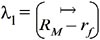 are not rejected at 5% significant level. It is concluded from second pass regression that SML which is upward sloping showing that the more risk is rewarded by more expected return, is supported. The reason behind such results can be partially explained by error in variable problem that is the betas calculated in first pass regression are not free of error.
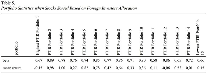
There is positive linear relationship between realized mean return and risk when stocks sorted based on percentage of foreign investor allocations is developed to test the hypothesis directly. We used the statistic for foreign investor that is the percentage rate in given stock holdings. We sorted stocks based on the total foreign allocation in given stocks and constructed 15 equal size portfolios for the purpose of testing the relationship between average portfolio returns and portfolios risk indicator, betas. Table 5 reports relevant statistics for testing the proposed hypothesis.
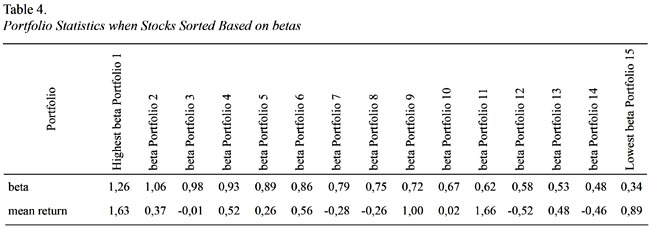
The reason behind testing hypothesis that there is a positive linear relationship between realized mean return and risk when stocks sorted based on their betas is simply to cluster stocks from high risk profile to low and observe a meaningful explanation to identify assumed relationship. Sorting procedure for testing hypothesis is not unique and one of the common ways used in literature. In doing so, we had fifteen (15) observations used in second pass regression depicted in Figure 11 for investigating risk return trade off. The portfolios constructed with ten stocks when stocks sorted from the one with highest beta to lowest except the last portfolio which consists of 14 stocks whose betas are lowest. Table 4 gives the relevant statistics for the procedure described.
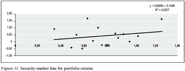
Results coming out from regression depicted in Figure 11 are not supportive for the assumed hypothesis. Even though beta coefficient is satisfactorily different than zero, the alpha coefficient is far away from theoretical value which is zero in equilibrium. The explained variation in portfolio mean return is just 5%, which is reflected by R Square statistics and relatively low when it is compared with the previous sorting procedure. The theoretical rational behind such results can be partially explained by the uniqueness of Turkish Capital Market microstructure. In other words, there might be other source of reason to cluster stocks within the portfolios. This is what we exactly did for testing the following hypothesis and sort the stocks based on the characteristics of investors.
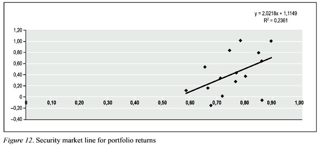
Results do not surprise us to figure out the role of one of the elements regarding the microstructure of Turkish Capital Market that is the foreign investors allocation. Regression output, which is depicted in Figure 12, is much more supportive in the favor of a positive linear relationship between risk and return. The beta coefficient is 2.2 implying that in the case of one percent increase in portfolio mean return, there would be 2.2% increase in risk and statistically significant. Alpha value is not zero but much lower than the alpha gained in previous investigation. The most important statistics here is that 23% R Square is quite well for a cross sectional regression analysis. We also explore the impact of an outlier (Figure 12) and take it out from the analysis. The results are much clearer for the assumed hypothesis and is depicted in Figure 13.
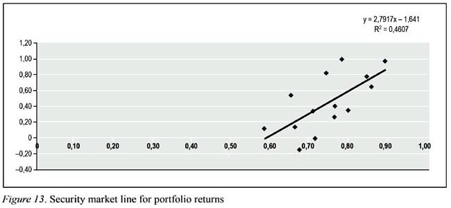
Regression output, as demonstrated in Figure 13, shows a clear picture for a meaningful explanation between risk and return. Explained variations in portfolio mean return in this case increased to 46% and lead us to conclude that such sorting procedure is much more meaningful to investigate risk return trade off.
Cross-sectional Investigations (2005 only )
Despite the fact that cross sectional investigation conducted through the 2002:01-2008:06 period gives us important inferences about cross sectional asset returns, there are certain limitations that lead us to employ yearbased analysis on portfolio returns. The main limitation is that accounting standards change over the period. Therefore, accounting based measures do not reflect the true value for given variables. For any accounting based variables, there is immeasurable component due to changes in accounting standards. Istanbul Stock Exchange database does report unstable financial statements, therefore, two consecutive years figures are not the same. For example, ISE database reports financial statements for 2005 and 2006 together and in the same manner for 2006 and 2007. However, the figures for 2006 in both reports may not be the same. Since investigation is made for all manufacturing firm, adjustments that are needed to fix financial statements are time consuming. As a results, cross sectional analysis through 2002:012008:06 is skipped due to the fact that year based cross sectional analysis is much more reliable.
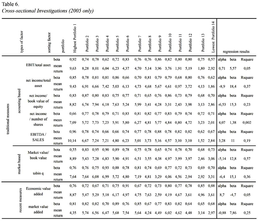
Table 6 reports portfolio based cross sectional asset return and risk trade off for 2005 only. The most regression results significant results coming from the analysis is market value/book value sorting procedure. This means that when we sort stocks based on market value/book value criteria and construct portfolios with equal number of stocks from the highest value to lowest, 57% of variation in portfolio average return can be explained by stocks systematic risk in 2005. The other significant results are net income/total asset with 37% R Square; Tobin q with 36%; Market Value Added with 25%; net income/book value of equity with 23%; and EBITDA/ Sales with 19%. However, Economic Value Added as a sorting factor does not lead positive risk return tradeoff relationship. When stocks sorted based on EVA, firms systematic risk and average returns seem to be negatively correlated which contradicting with a fundamental inference for the given year.
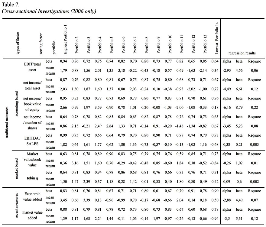
Cross-sectional Investigations (2006 only)
Table 7 reports portfolio based cross sectional asset return and risk trade off 2006 only. The most significant results coming from the analysis is net income/book value of equity value sorting procedure. This means that when we sort stocks based on net income/book value of equity criteria and construct portfolios with equal number of stocks from the highest value to lowest, 22% of variation in portfolio average return can be explained by stocks systematic risk in 2006. The other significant results are net income/total asset with 12% R Square; and Market Value Added with 12%. These results show that explained variations in portfolio returns are less in 2006 than in 2005, whereas all sorting factors do lead positive risk return trade off relationship. When stocks sorted based on these sorting factors, firms systematic risk and average returns seem to be positively correlated which is not contradicting with a fundamental inference for the given year.
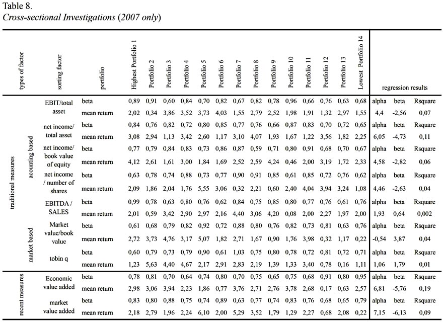
Cross-sectional Investigations (2007 only)
Table 8 reports portfolio based cross sectional asset return and risk trade off for 2007 only. The most significant results coming from analysis is Economic Value Added sorting procedure. This means that when we sort stocks based on Economic Value Added criteria and construct portfolios with equal number of stocks from the highest value to lowest, 19% of variation in portfolio average return can be explained by stocks systematic risk in 2007. The other significant results are net income/total income/book value of equity, net income / number of shares, Economic Value Added and market value added as sorting factors do not lead positive risk return tradeoff relationship. When stocks sorted based on these sorting factors, firms systematic risk and average returns seem to be negatively correlated which is contradicting with a fundamental inference for the given year.
CONCLUSION
We developed and tested investigations for cross sectional stock returns in light of neoclassical and behavioral asset pricing models. The results, explained in detail in previous sections, are preliminaries implying that there are primitive and not strictly underlined for the fact that accounting data may produce bias in any such empirical studies. The most important limitation is that there is no linkage made between taxes and stock returns. It is an important limitation for the fact that the total number of foreign investors might be different if taxes are not the same for both foreign and local investors. An investor is classified as foreigner if the account is opened in a different country than Turkey. We used simple econometric techniques to investigate the derived hypothesis and panel data analysis is needed to explore the other role of factors, whereas it seems not possible to apply panel data analysis due to the inconvenient accounting figures in Turkey. However, the implications for future research raised by the present paper are the extremely significant questions: (i) what is the role of foreign investors allocation in testing the market efficiency of Turkish Capital Market in general, and (ii) in testing asymmetric information in particular. Such questions require academics to deal with in depth analysis with data transformation and econometric techniques, whereas economically meaningful explanations are needed to develop a general theory for financial markets in general, and for emerging markets in particular.
REFERENCES
Arnold, G. (1998). Corporate Financial Management. London: Pitman Publishing.
Armitage, H. M., & Fog, V. (1996). Economic Value Creation: What Every Management Accountant Should Know. CMA Magazine, October, 21-24.
Aslanertik, B. E. (2007). Enabling Integration to Create Value through Process-Based Management Accounting Systems. International Journal of Value Chain Management, 1(3), 223 – 238.
Bacidore, J. M., Boquist, J. A., Milbourn, T. T., &. Thakor, A.V. (1997). The Search for the Best Financial Performance Measure. Financial Analysts Journal, 53(3) May/June, 11-20.
Biddle, G. C., Bowen, R. M., & Wallace, J. S. (1997). Does Eva Beat Earnings? Evidence on Associations With Stock Returns and Firm Values. Journal of Accounting and Economics, 24(3), 301-336.
Celik, S., Aktan, B., & Mandaci, P. E. (2008). The Characteristics of Bank Common Stocks within the Framework of Capital Asset Pricing Model: Evidence from Turkey. Investment Management and Financial Innovations, 5(4), 157-172.
Celik, S., Mandaci P. E., & Cagli,, E.C. (2009). An Examination of Risk and Return Trade off in Manufacturing Industry: An Asset Pricing Approach. Middle Eastern Finance and Economics, 4(September), 5-27.
Celik, S., Mandaci P. E., Masood, O., & Aktan, B. (2009). The Linkages between Characteristics of Investors and Stock Returns: An Empirical Inquiry in Istanbul Stock Exchange. Paper presented at 5th International Conference on Business, Economics and Management, Izmir, Turkey.
Chen, S., & Dodd, J. L. (2001). Operating Income, Residual Income and EVA: Which Metric is More Value Relevant? Journal of Managerial Issues, 13(1), 65-86.
Chung, K. H., & Pruitt, S. W. (1994). ASimple Approximation of Tobins q. Financial Management, 23(3), 70-74.
Clinton,, B. D., & Chen. S. (1998). Do New performance Measures Measure Up? Management Accounting, (October), 38, 40-43.
Cochrane, J. H. (2005). Asset Pricing, (Rev. Ed.). New Jersey: Princeton University Press.
Ehrbar, A. (1998). Economic Value Added: The Real Key to Creating Wealth. New York: John Wiley & Sons, Inc.
Grant, J. L. (1996). Foundations of EVA for Investment Managers. The Journal of Portfolio Management, 23(Fall), 41-48.
Lehn, K., & Makhija, A. K. (1997). EVA, Accounting Profits and CEO Turnover: An Empirical Examination 1985-1994. Journal of Applied Corporate Finance, 10(2), 90-97.
Lindenberg, E. B., & Ross, S. A. (1981). Tobin q Ratio and Industrial Organization.. Journal of Business, 54(1), 1-32.
Lintner, J. (1965). The Valuation of Risk Assets and the Selection of Risky Investments in Stock Portfolios and Capital Budgets. Review of Economics and Statistics, 47(1), 13-37.
Marsh, D. G. (1999). Making or Breaking Value. New Zealand Management, March, 58-59.
Mehra, R., & Prescott, E. C. (1985) . The Equity Premium: A Puzzle. Journal of Monetary Economics, 15, 145−161.
Merchant, K., & Sandino, T. (2009). Four Options for Measuring Value Creation. Journal of Accountancy, August, 34-37.
Modigliani, F., & Miller, M. (1963). Corporate Income Taxes and the Cost of Capital: a Correction. American Economic Review, 53(3), 433–443.
ISE (2008). Sermaye Piyasası ve Borsa Temel Bilgiler Kılavuzu. 20e, Nisan. Retrieved from <http://imkb.gov.tr/yayinlar/spkilavuzu.htm>.
Perfect, S. B., & Wiles, K. W. (1994). Alternative Construction of Tobins q: An Empirical Comparison. Journal of Empirical Finance, 1(3/4 July), 313-41.
Peterson, P. P., & Peterson, D. R. (1996). Company Performance and Measures of Value Added. Short Hills, NJ: The Research Foundation of the Institute of Chartered Financial Analysts.
OByrne, S. F.(1996). EVA and Market Value. Journal of Applied Corporate Finance, 9(1 Spring), 116-125.
Rappaport, A. (1986). Creating Shareholder Value. (1st. Ed.). New York: The Free Press.
Rappaport, A. (1998). Creating Shareholder Value. (2nd. Ed.) New York: The Free Press.
Ray, R. (2001). Economic Value Added: Theory, Evidence, a Missing Link. Review of Business, 22(1/2), 66-70.
Ronte, H. (1998). Value based management. Management Accounting: Magazine for Chartered Management Accountants, 76(1), 38-39.
Sharpe, W. F. (1964). Capital Asset Prices: A Theory of Market Equilibrium under Conditions of Risk. Journal of Finance, 19(4), 425-42.
Simms, J. (2001). Marketing for Value. Marketing, 28(June), 34-35.
Stewart, G. B. (1991). The Quest for Value, New York: Harper Business.
Stewart, G. B. (1994). EVA: Fact and Fantasy. Journal of Applied Corporate Finance, 7(2), 71-84.
Uyemura, D. G., Kantor, C. C., & Petit, J. M. (1996). EVA for Banks: Value Creation, Risk Management and Profitability Measurement. Journal of Applied Corporate Finance, 9(2), 94-111.
Xavier, A., & Pere, V. (2003). FEVA: A Financial and Economic Approach to Valuation. Financial Analysts Journal, 59(2), 80-87.
Yook, K. C., & McCabe, G. M. (2001). MVA and the Cross-section of Expected Stock Returns. Journal of Portfolio Management, 27(3), 75-87.
Walbert, L. (1994). The Stern Stewart Performance 1,000: Using EVA to Build Market Value. Journal of Applied Corporate Finance, 6(4), 109-112.
-
Mehra and Prescott (1985) were the first to introduce the equity primium puzzle. This is what Cochrane emphasizes.
-
Such way of thinking is just a simplification of a complex reality as if how it is done through celebrated model of asset pricing, Capital Asset Pricing Model (CAPM).
-
By price we mean that the price on which transaction is en ded. The ending price can be also defined as market price.
-
By value we mean that the real value, despite the fact that it is hardly quantified. The real value can also be defined as intrinsic value.
-
Price-Value Equilibrium is achieved when discount rate for a given asset is equal to its required rate of return.
-
Celik et al. (2009) pointed out that the remarkable question that should be answered is what the role of this increase is on cross sectional stock returns. First and foremost, the underlining point is that if there is statistical significant difference between stock returns that are traded by foreign investors and local investors, we can ask if there is a role of asymmetric information. In other words, is the market efficiency scale up or down by the trading of foreign investors?
-
In the market model framework, the regression is employed for each asset with Ordinary Least Square algorithm. This procedure is conducted as in Celik et al. (2008, 2009).
Received: March 3, 2011
Accepted: July 7, 2011
