ARTICLE

 

Is gold a hedge or a safe haven? An application of ARDL approach

 

Mohammad Hassan Shakil¹; Is’haq Muhammad Mustapha²; Mashiyat Tasnia³; Buerhan Saiti⁴

¹International Centre for Education in Islamic Finance, Kuala Lumpur, Malaysia and Taylor’s University, Subang Jaya, Malaysia
²International Centre for Education in Islamic Finance, Kuala Lumpur, Malaysia
³International Islamic University Malaysia, Kuala Lumpur, Malaysia
⁴Istanbul Sabahattin Zaim University, Istanbul, Turkey

 

---

Abstract

Purpose – The argument whether gold is a hedge or haven is a debatable issue. Mainly, hedge is a class of asset that is negatively correlated with another asset or portfolio on average. On the other hand, a safe haven is an asset or portfolio which is negatively correlated with another asset or portfolio at the time of market turmoil. Therefore, the purpose of this research is to take Saudi Arabia as an example to examine the relationship of gold price in Saudi Arabia with key determinants such as the stock market index, oil prices, exchange rate, interest rate and consumer price index (CPI) by application of the autoregressive distributed lag model (ARDL).
Design/methodology/approach – The ARDL analysis was employed by using six variables based on the application of monthly time series data that were collected from 2011 to 2015.
Findings – From the present analysis, it has been discovered that gold is useful as a portfolio hedge and as a hedge against inflation because it is not affected by the CPI. External factors, for example, financial crisis, may be harmful to the CPI, thus adding a certain percentage of gold in the investment portfolio may assist in decreasing the level of risk at the time of financial turmoil.
Originality/value – Because gold seems to be a useful portfolio hedge, as well as an inflation hedge, government policies to curb the import of gold may be futile. The present research suggests that policies that directly address the causes of inflation and provide alternative investment opportunities for retail investors may better serve the objective of decreasing gold imports.

Keywords ARDL, Oil price, Gold price, Islamic stocks

 

---

1. Introduction

Despite the recent fall in the prices for general commodity, investing in commodities has a benefit that is better than most other financial assets, when considering the fact that commodities are divided into two types, hard and soft commodities. The hard commodities are natural resources that must be mined or extracted (such as oil, rubber and gold), while soft commodities are agricultural products or livestock (such as corn, wheat, sugar, coffee, soybeans and pork). According to researchers, diversification benefits can be achieved through investing across sectors and across countries; however, in the current homogenization and co-movement of global financial system, investors must be alert that the correlation among the sectors is dynamic, which can change sharply with a certain event. Therefore, it is better to invest in an asset that ideally contained either low or negative correlations with each other. In the case of an investment, we do not know the interest rates in the future, which can be either high or low. Similarly, we do not know which asset category, i.e. real estate, gold, stocks or bonds, will outperform or underperform in the future. Which business industry or sector will outperform in the future? Will mining and oil stocks outperform or will it be utilities, pipelines and communications? Because of these unknown circumstances, to make an investment effective, a portfolio must be carefully planned. The portfolio plan should note that the future will not at all the times unfold as expected; the methodology must be flexible enough to enable adjustments according to circumstances.

Among every single precious metal and the most popular choice for investment, gold stands out. It has passed the test of time, and it has performed well amid crisis situations such as market decline, currency failure, high inflation, war, etc. Gold is primarily used in the production of jewelry, coins, medals, electronic components and so on. However, it is also used as an investment to defend real value against inflation, financial crisis and other uncertainties by governments, institutions and individuals worldwide (Wang et al., 2011; Thanh, 2015). In view of uncertainty of the world economy, the monetary market shows gold as an ideal inflation hedge and a portfolio holding. Most individual and institutional investors include gold in their portfolio to maintain a balance between the soft and physical assets. Furthermore, to manage the exchange rate and reduce the volatility, as well as enhance the risk and return balance, many central banks incorporate gold in the currency basket and reserve the asset portfolio, respectively.

However, the argument whether gold is a hedge or a haven is a debatable issue. Mainly, a hedge is a class of asset that correlates negatively with another asset or portfolio on average (Baur and Lucey, 2010). It does not have the power to reduce losses during times of market turmoil. On the other hand, a safe haven is an asset or a portfolio that correlated negatively with another asset or portfolio at times of market turmoil. The main attribute of a safe haven asset is the negative correlation with a portfolio in an extreme market condition. An asset is not forced to be negative or positive, on average. It will be only zero or negative during specific periods. So, in the normal market condition, the possibility of a correlation can be either positive or negative. At the time of adverse market conditions, if the haven asset is negatively correlated with other assets or portfolios, then the possibility of compensating the investor for the losses is higher. The reason for the compensation is that the price of the haven asset increases the minute the price of the other asset or portfolio decreases (Baur and Lucey, 2010). Many studies have assessed the pattern of gold prices (Capie et al., 2005; Worthington and Pahlavani, 2007; Baur and Lucey, 2010) to identify the factors that influence gold prices. The factors that play an influential role in the change in gold prices include inflation, exchange rate, bond prices, market performance, seasonality, income, oil ARDL approach 61 prices and business cycles. However, to the best of our knowledge, no study has examined gold prices in Saudi Arabia yet.

We performed an analysis to study the factors influencing gold prices in Saudi Arabia by collecting monthly data on gold prices and other factors over the period of 2011 to 2015. Although the hedge factors are expected to work in Saudi Arabia as in other countries, gold may not be relevant elsewhere and has previously overlooked in the literature. Saudi Arabians buy gold not just for investment but also for personal reasons, to use as a luxury good. If the abovementioned reasons are substantial, then higher affordability of individual citizen should lead to puffed-up demand and hence higher prices for gold. Moreover, we capture the wealth effect through the domestic Shariah price index of Saudi Arabia. The time-series variables that we study are, largely, non-stationary variables. For that reason, we should analyze them in a cointegrating framework. By applying the autoregressive distributed lag (ARDL) approach, we found that the gold price has a cointegrating relationship with the interest rate (INTR), consumer price index (CPI) and oil price (OILP). Further, we discover that gold is both a portfolio hedge and a hedge against inflation because it is free from the effect of the CPI. External factors, for example, financial crisis may be harmful to the CPI, thus adding some percentage of gold in the investment portfolio may assist in reducing the risk during a financial crisis.

Owing to the frequent economic crises of late, many international investors have been hurt and are weary of investing in equities. Since then, they have been searching for alternative asset classes as part of a diversified portfolio of investments, for example, commodities, to fulfil the need to maintain some level of returns, while not investing in high-risk securities (Saiti et al., 2014). Despite the immense importance of gold, there is insufficient empirical evidence on the relationship between gold and other commodities, i.e. the stock market index, oil prices, exchange rate, interest rate and consumer price index. Moreover, most studies have been conducted from only an international perspective, while little attention has been paid from a domestic point of view. Besides, previous literature on the subject is scarce, and findings are inconsistent. We believe that the study will fill the gap in the literature by using monthly data and applying the ARDL analysis. Our study has economic implications for academicians, policymakers, portfolio managers and risk hedgers. It will provide better insights of when and at which time horizon the gold can act best as a hedge, which provides a decision aid for better asset allocation of one’s portfolio.

The remaining discussion is depicted as follows: Section 2 explains the existing literature on gold as a hedge and a safe haven and the relationship between gold and other related variables. Section 3 describes the methodology and data. Section 4 presents the results, and Section 5 concludes the paper.

2. Literature review

In the case of making investment in commodities as this paper is trying to suggest, according to Bhardwaj and Dunsby (2013), researchers that support commodity investment typically refer to its overall low correlation with other asset classes, which is one of the main three benefits of investing in the commodity market. The other two benefits are its similarity with equity in the case of returns and its positive correlation with inflation. In the most recent 50 years, the stock–commodity correlation has been near zero, in which their annual correlation ranged from _0.39 to 0.76.

According to Frush (2008), investing in commodities can produce excellent results that investors are looking to achieve, especially those who want to gain an edge. Investing in commodities provides many advantages and benefits that are not accessible with conventional stock and bond investment. Wise investors know the advantages of allocating to fundamentally different asset classes such as commodities. In the event that an investor does not invest in commodities, he or she will form a suboptimal portfolio in which there are lower return possibility and higher risk levels, leading to a loss.

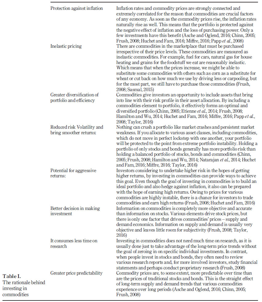
Several research studies concentrate on how people should allocate their investments instead of which individual investments they should select or when they should purchase them and sell them as the main determinant of investment performance over time. But by allocating even a small percentage of portfolios to commodities, it will improve the risk and return profiles of the portfolio. This means that your portfolio will be better positioned to weather stock market declines, will be safeguarded against huge fluctuations in the total portfolio value and will have greater opportunities for higher performance over time. Table I summarizes the reasons why investors should invest in commodities gathered in this research paper from many researchers (Asche and Oglend, 2016; Chinn, 2005; Frush, 2008; Hamilton andWu, 2014; Huchet and Fam, 2016; Miffre, 2016; Papp et al., 2008; Taylor, 2016).

Among the commodities, gold has been considered as a safe haven for a long period of time. But the hypothesis that gold is a safe haven has not been formally tested until recently. Baur and Lucey (2010) defines the terms hedge and haven and tests whether gold is a hedge or a safe haven by using daily data collated from 1995 to 2005. They mainly analyzed the role of gold as a safe haven asset with respect to the stock market movement. They reported that gold holds its value in the USA, the UK and Germany, on average, when the stock markets experiences adverse negative returns. Based on their findings, gold acts as a safe haven for a certain time period, around 15 trading days. In addition to that, Baur and McDermott (2010) examined the role of gold as a safe haven against equities of developed and major emerging markets. They used data from 1979 to 2009 and showed that gold was both a hedge and a safe haven for major European and the US Stock Markets but not for the stock markets in Australia, Canada, Japan and major emerging markets such as BRIC countries (Brazil, Russia, India and China). Furthermore, Ibrahim (2012) studied the relationship between gold and stock market returns from the perspective of Malaysia. He checked the variability of gold and stock market returns during the consecutive negative market returns by applying the autoregressive distributed model to link the gold returns to stock returns with TGARCH/EGARCH error specification. He used daily data collated from August 2001 to March 2010 and found that there is a significant positive but low correlation between gold and stock returns. Further, he explained that the gold market surges when it faces consecutive market declines. Moreover, Ciner et al. (2013) examined the relationship of returns with five selected financial asset classes to determine whether these classes of assets can be considered as a hedge or a safe haven against each other. By using the daily data set from the UK and the USA for the period between 1990 and June 2010, they found that gold can be considered as a safe haven against the exchange rates of both countries.

On the other hand, Hiller et al. (2006) examined the role and effect of gold and other commodities in the equity markets. They used the data collated between 1976 and 2004 and found that gold has a small negative correlation with the S&P500 Index. In addition to that, it was found that the portfolio with gold performed better than the portfolio without gold. Similarly, Ziaei (2012) uses the generalized method of moments (GMM) model to analyze the effects of gold price on equity, bond and domestic credit in the ASEANþ3 countries (Indonesia, Malaysia, the Philippines, Singapore, Thailand, China, Japan and South Korea) from 2006 to 2011. The results indicate that the gold price significantly influences the bond and equity market, that is, any negative changes in equity market will have positive effects on the gold price. Comparably, Garefalakis (2018) examined the effect of gold on the Hang Seng Index series by applying the GJRGARCH model for the period between 2002 and 2009 and discovered that gold has a negative relationship with equity prices. After using the cointegration regression technique on monthly gold price from 1976 to 1999, Ghosh et al. (2004) found that the rise in gold price over time at the general level of inflation. He further explained that it is an effective hedge against inflation. On the other hand, the deviations in real interest rate, gold lease, exchange rate, default risk and covariance of the return of gold with other assets disrupt the short-run equilibrium relationship. Moreover, it generates volatility of the short-run price.

There is not enough empirical evidence of gold and its impact on other variables. The study will try to fill the gap in the literature by applying the ARDL approach by using recent monthly data. For academicians, it would provide better insights. Later they can depict when and in which time horizon the gold can best act as a hedge. From the perspective of investors, this would provide a decision aid for healthier allocation of one’s portfolio.

3. Methodology

The paper depicts the nature of the relationship of gold price in Saudi Arabia with key determinants such as the Shariah-compliant stock market index, oil price, exchange rate, interest rate and consumer price index by applying theARDL analysis on monthly time series data from 2011 to 2015.

The empirical model is given by:

where:
GLDP = gold price in US$;
ESTIC = S&P Saudi Arabia Domestic Shariah Price Index;
INTR = interest rate – government, securities and Treasury bills;
EXR = exchange rate;
CPI = consumer price index; and
OILP = OPEC oil basket price US$/barrel.

The time series techniques methodology–ARDL co-integration approach is used first to test the existence of a long-term relationship with the lagged levels of the variables. It helps to identify the dependent variables (endogenous) and the independent variables (exogenous). More so, if the relationship among the variables is long term, then the ARDL analysis creates the error-correction model (ECM) equation for every variable, which provides information through the estimated coefficient of the error-correction term about the speed at which the dependent variable returns to equilibrium once it is shocked. The ARDL model specifications of the functional relationship between gold price (in US$) (GLDP), S&P Saudi Arabia Domestic Shariah Price Index (ESTIC), interest rate (INTR), exchange rate (EXR), CPI, OPEC oil basket price US$/barrel (OILP) can be estimated in equation (2):

 

where k = lag order (Need to clarify if 1 is good)

ARDL-bound testing procedure permits us to take into consideration I(0) and I(1) variables together. The null hypothesis of the non-existence of a long-run relationship which is denoted by F_LGLDP(LGLDP|LESTIC, LINTR, LEXR, LCPI, LOILP) and the other components of equation (2) are denoted as follows:

These are tested against the alternative hypothesis of the existence of co-integration:

 

The calculated F-statistics derived from theWald test are compared with Pesaran et al.’s (2001) critical values. If the calculated F-statistics falls below the lower-bound critical values, then we fail to reject the null hypothesis of the non-existence of a long-run relationship. Moreover, if the calculated F-statistic lies between the lower- and upper-bound critical values, then the result is inconclusive. On the other hand, if the calculated F-statistics is more than the upper-bound critical values, then we reject the null hypothesis "non-existence of a long-run relationship".

Once the existence of a long-run relationship between variables is valued, the next step is to select the optimal lag length by using standard criteria such as Schwarz Bayesian criterion (SBC) or Akaike Information (AIC). Only after the test can the long- and short-run coefficients be predicted. The ARDL long-run form is exhibited in equation (3):

 

The error-correction term which was used in the ARDL short-run model to depict the short run dynamics is shown in equation (4):

where, ECT = lagged error-correction term. We will be testing the null hypothesis (H₀) of the "non-existence of the long-run relationship" against the alternative of "the existence of the long-run relationship"

H0=b1=b2=b3=b4=b5=b6=0

H1=b1≠b2≠b3≠b4≠b5≠b6≠0

Logarithmic transformations of all variables were calculated to achieve stationarity in variance. Thereafter, we began empirical testing by determining the stationarity of all variables in our consideration. This is necessary to proceed with the testing of the cointegration later. Ideally, our variables should be I(1), in that they only become stationary after their first difference. The differenced form for each variable used is created by taking the difference of their log forms (e.g. DGLDP = LGLDP- LGLDP_t-1).

4. Findings and interpretations

4.1 Unit root test

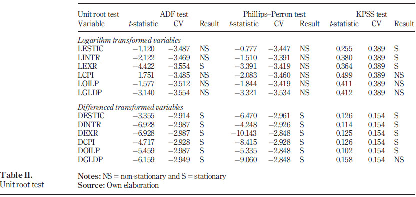
We then conducted the Augmented Dickey–Fuller (ADF), Phillips–Perron (PP) and Kwiatkowski–Phillips–Schmidt–Shin (KPSS) test. The ADF tests each variable (in both level and differenced form). A stationary series has a mean, a finite variance, shocks are transitory and autocorrelation coefficients die out as the number of lags grows, while a nonstationary series has an infinite variance, shocks are permanent and its autocorrelations tend to be a unity.

The outcomes of the unit root test vary from one test to another. If we examine the results of the unit root tests for all variables in the level and differenced forms, we see that in the level form, the exchange rate (EXR) shows a different result in the ADF and PP tests; however, in the KPSS test, it shows that most of the variables are stationary except the gold price in a differenced form. Thus, the results are not consistent across various tests. Therefore, we are using variables I(0) or I(1) for the analysis.

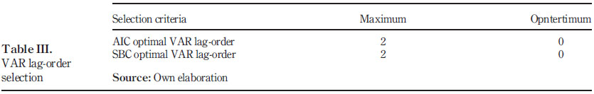
The results of the unit root test are not consistent, as our variables are found to be a mixture of I(0) and I(1), and the results show different results in each test as shown in Table II. Therefore, we decided to use the ARDL technique to test the long-run relationship among the variables. Before proceeding with the test of co-integration, we try to determine the order of the vector autoregression (VAR), that is, the number of lags to be used. It is, however, not necessary to find the VAR order for the ARDL approach, as the process itself finds the individual lag order for each variable.

Similarly, as we have monthly data and the observation is 64 data points, we assume a maximum of 2 VAR orders, which are as shown in Table III, and both AIC and SBC recommend no lag order. This can be interpreted as inherent nature of the time-series data of our study. This is a limitation that can be overcome using the ARDL technique, which determines the specific lag order for each variable in our investigation.

4.2 Testing for co-integration

Evidence of co-integration implies that the relationship between the variables is not spurious, i.e. there is a theoretical relationship among the variables and that they are in equilibrium in the long run.

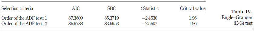
As depicted in Table IV, the critical value is less than the t-statistic value. So, we reject the null that the residuals are non-stationary. Statistically, the aforementioned results indicate that the variables we have chosen, in some combination, result in a stationary error term. The stationarity of the error term indicates that there is co-integration among variables. These initial results are intuitively appealing to our mind. On the other hand, if the variables are not found to be co-integrated, they may be fractionally co-integrated. For furtherance to this result, we decided to go for the Johansen cointegration test.

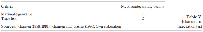
4.2.1 Johansen co-integration test. As depicted in Table V, the maximal eigenvalue and trace of the stochastic matrix show one and two cointegrating vectors, respectively, which are somewhat contradictory.

The implication of the co-integration results above is that each variable contains information for the prediction of other variables. However, these results are in conflict with each other; it is also in conflict with the results of the study by Engle and Granger (1987). So far, we have seen that these approaches have many limitations that question the robustness of the techniques. We believe that the limitations can be taken care of by using the Standard ARDL technique. As such we have decided to go for the ARDL approach with the robust approach for testing co-integration among variables.

Table VI shows that the calculated F-statistics for variables DESTIC (S&P Saudi Arabia Domestic Shariah Price Index) is 4.1053, which is higher than the upper-bound critical value of 3.646 at the 5 per cent significance level.

 

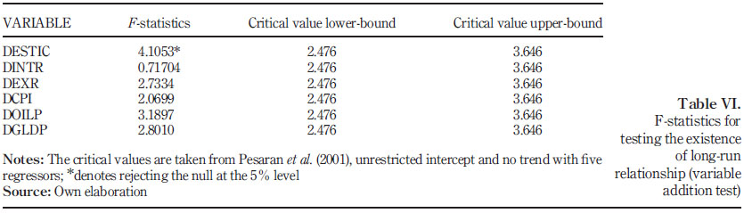
This implies that the H0 of the non-existence of a co-integrating long-run relationship" can be rejected. These results reveal that a long-run relationship exists in variables. This could be considered as a finding in view of the fact that the long-run relationship between the variables is demonstrated here, avoiding the pre-test biases involved in the unit root tests and cointegration tests required in the standard co-integration procedure. The evidence of the long-run relationship rules out the possibility of any spurious relationship between the variables. In other words, there is a theoretical relationship between the variables. However, there is need to confirm the endogeneity and exogeneity of variables. At this stage, we run the ARDL test to confirm the short- and long-term relationship and study long-run coefficients and ECM to identify which variables are endogenous and which are exogenous.

4.3 Long-run coefficient estimation

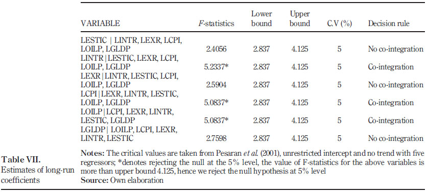
From Table VII, we find that when the gold price (GLDP) is the dependent variable, the calculated F-statistic LGLDP| LOILP, LCPI, LEXR, LINTR, LESTIC = 2.7598 is less than the upper bound of the critical value obtained from Pesaran et al. (2001), indicating that there is no significant evidence for co-integration between the gold price and its determinant in Saudi Arabia for the study period. However, the evidence of the long-run relationship rules out the possibility of any spurious relationship between the variables. In other words, there is a theoretical relationship between the variables. The process has been repeated for other variables, and the result shows that the interest rate (INTR), CPI and oil price (OILP) indicate compelling evidence of a long-run relationship with the determinants.

4.4 Error-correction model of ARDL

In Table VIII, ECM’s representation for the ARDL approach is selected using the SBC criterion.

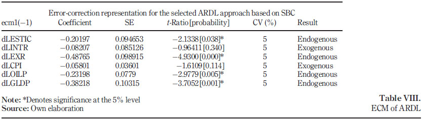
The error-correction coefficient estimated for exchange rate (EXR) and gold price (GLDP) is _0.49(0.10) and _0.38(0.10) respectively, which is insignificant, has a negative sign and implies a slow speed of adjustment to equilibrium after a shock. The errorcorrection coefficient estimated for interest rate (INTR) and CPI at _0.08(0.09) and _0.06 (0.04), respectively, is highly significant, has the correct sign and implies existence of a medium- to long-term adjustment to equilibrium after a shock. Finally, the "t" or "p" value of the coefficients of the Δ (i.e. differenced) variables indicate whether the effects of these variables on the dependent variables are significant in the short run.

Furtherance to this, we can argue that vector error correction model (VECM) has given a clear picture of the short- and long-run relationship among variables; with regard to our research objective, VECM shows that three of our variables are endogenous and the other two are exogenous, that is, nearly half of these variables are dependent on other variables, while the remaining half are independent of other variables. Although the ECM tends to indicate the endogeneity/exogeneity of a variable, it does not indicate the relative degree of endogeneity or exogeneity. As such, we had to apply the variance decomposition (VDC) technique to discern the relative degree of endogeneity or exogeneity of the variables.

4.5 Variance decompositions

The relative exogeneity or endogeneity of a variable is determined by the proportion of the variance explained by its own past (Domingos, 2000). The analysis aims at calculating the contribution of innovations to the forecast-error variance. To that effect, we express the individual forecast-error variance to a given horizon in a function of the error variance assigned to each variable in the system to obtain the relative importance of percentage. The results of data collected over a 48-month horizon is presented in Table VIII. It indicates the extent to which the individual forecast-error variance of any variable is explained largely by its own variations. It is worth stressing that the contributions are identical for the variables in the earlier periods and later over the 48-month horizon. Another feature of substantial importance is that all the variables almost contribute to the forecast-error variance of any variable, implying that there are cross-effects between the variables. The variable that is explained mostly by its own shocks (and not by others) is deemed as the most exogenous of all. We started out by applying generalized VDCs and obtained the results which are presented in Figure 1.

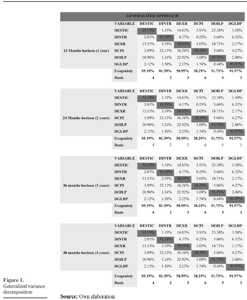
The results indicate that gold is found to be the most exogenous, and thus, it depends mostly on its own as compared to other variables. We also can see that the most follower or most endogenous is the CPI. Therefore, the gold price is not affected by the CPI, while, the drop in the gold price can be predicted as "bad luck" for the financial sector. From the perspective of an investor, we might say that gold can be a hedging for inflation, as it is not affected by the CPI. External factors, for example, the financial crisis, may be harmful to the CPI, thus adding some percentage of gold in the investment portfolio may assist to reduce the risk in the event of financial crisis.

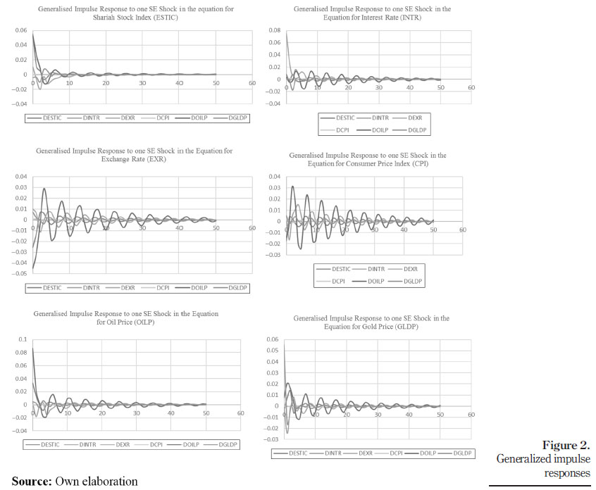
4.6 Impulse response

Impulse response (IR) analysis is based on the VAR model, which is shown in Figure 2. It is not a necessary step for the ARDL method. ARDL does not need to fulfil the series, that is, I (0) and I(1), while VAR requires this precondition to carry out all other steps.

The advantages of the IR analysis include the fact that it provides policymakers with additional information about which variable is the most exogenous and about relative exogeneity/endogeneity. Therefore, policy makers will monitor the variable which is the most exogenous for achieve the economic target. Moreover, the impulse response functions essentially produce the same information as the VDCs, except that they can be presented in a graphical form. If any specific variable was shocked, we will see the immediate effect on others.

 

5. Conclusion

We have depicted the gold prices in Saudi Arabia and shown it to have a long-time relationship with the interest rate, the CPI and oil prices. Gold prices are negatively related to oil prices, which indicate the role of gold as a hedge. Gold prices go up when the Saudi Riyal is weaker, implying that gold is a good hedge against the dollar. When returns from investing outside the country are high, gold prices in Saudi Arabia are low. Finally, gold acts as a good inflation hedge, as it moves in the same direction as CPI. Because gold seems to be a useful portfolio hedge and an inflation hedge, government policies to curb the import of gold may be futile. Our research suggests that policies that directly address the causes of inflation and provide alternative investment opportunities for retail investors may better serve the objective of bringing down gold imports.

Future work in this area can proceed in several directions. In terms of methodology, alternative approaches such as copula, artificial neural networks, Fourier transformation and wavelet analysis can be used to assess the scope for improvement in the forecasting power. Other research approaches such as behavioral finance models can be tested using micro data on investors’ personal choices to study their influence on gold prices. Studies can compare the gold holding decisions of households and corporate houses to evaluate the consumption vis-à-vis investment motives behind the gold purchase.

 

References

Asche, F. and Oglend, A. (2016), "The relationship between input-factor and output prices in commodity industries: the case of Norwegian salmon aquaculture", Journal of Commodity Markets, Vol. 1 No. 1, pp. 35-47.

Baur, D.G. and Lucey, B.M. (2010), "Is gold a hedge or a safe haven? An analysis of stocks, bonds and gold", Financial Review, Vol. 45 No. 2, pp. 217-229.

Baur, D.G. and McDermott, T.K. (2010), "Is gold a safe haven? International evidence", Journal of Banking& Finance, Vol. 34 No. 8, pp. 1886-1898.

Bhardwaj, G. and Dunsby, A. (2013), "Of commodities and correlations", Journal of Indexes, available at: www.indexuniverse.com/publications/journalofindexes/joi-articles/19085-of-commodities-andcorrelations.html

Capie, F., Mills, T.C. and Wood, G. (2005), "Gold as a hedge against the dollar", Journal of International Financial Markets, Institutions and Money, Vol. 15 No. 4, pp. 343-352.

Chinn, M.D. (2005), "The predictive content of energy futures: an update on petroleum, natural gas, heating oil and gasoline (No. w11033)", National Bureau of Economic Research.

Ciner, C., Gurdgiev, C. and Lucey, B.M. (2013), "Hedges and safe havens: an examination of stocks, bonds, gold, oil and exchange rates", International Review of Financial Analysis, Vol. 29, pp. 202-211.

Domingos, P. (2000), "A unified bias-variance decomposition for zero-one and squared loss", 7th National Conference on Artificial Intelligence (1999), Washington, pp. 564-569.

Engle, R.F. and Granger, C.W.J. (1987), "Co-integration and error correction: representation, estimation, and testing", Econometrica: Journal of the Econometric Society, Vol. 55 No. 2, pp. 251-276.

Etienne, X.L., Irwin, S.H. and García, P. (2014), "Bubbles in food commodity markets: four decades of evidence", Journal of International Money and Finance, Vol. 42, pp. 129-155.

Frush, S. (2008), Commodities Demystified, McGraw Hill Professional, New York, NY.

Garefalakis, A., Dimitras, A., Spinthiropoulos, K.G. and Koemtzopoulos, D. (2018), "Determinant factors of Hong Kong stock market", International Journal of Finance and Economics, available at SSRN: https://ssrn.com/abstract=2200671

Ghosh, D., Levin, E.J., Macmillan, P. and Wright, R.E. (2004), "Gold as an inflation hedge?", Studies in Economics and Finance, Vol. 22 No. 1, pp. 1-25.

Hamilton, J.D. and Wu, J.C. (2014), "Risk premia in crude oil futures prices", Journal of International Money and Finance, Vol. 42, pp. 9-37.

Hiller, D., Draper, P. and Faff, R. (2006), "Do precious metals shine? An investment perspective", Financial Analysts Journal, Vol. 62 No. 2, p. 98.

Huchet, N. and Fam, P.G. (2016), "The role of speculation in international futures markets on commodity prices", Research in International Business and Finance, Vol. 37, pp. 49-65.

Ibrahim, M.H. (2012), "Financial market risk and gold investment in an emerging market: the case of Malaysia", International Journal of Islamic and Middle Eastern Finance and Management, Vol. 5 No. 1, pp. 25-34.

Johansen, S. (1988), "Statistical analysis of cointegration vectors", Journal of Economic Dynamics and Control, Vol. 12 Nos 2/3, pp. 231-254.

Johansen, S. (1991), "A Bayesian perspective on inference from macroeconomic data: comment", Scandinavian Journal of Economics, Vol. 93 No. 2, pp. 249-251.

Johansen, S. and Juselius, K. (1990), "Maximum likelihood estimation and inference on cointegration – with applications to the demand for money", Oxford Bulletin of Economics and Statistics, Vol. 52 No. 2, pp. 169-210.

Miffre, J. (2016), "Long-short commodity investing: a review of the literature", Journal of Commodity Markets, Vol. 1 No. 1, pp. 3-13.

Natarajan, V.K., Singh, A.R.R. and Priya, N.C. (2014), "Examining mean-volatility spillovers across national stock markets", Journal of Economics Finance and Administrative Science, Vol. 19 No. 36, pp. 55-62.

Papp, J.F., Bray, E.L., Edelstein, D.L., Fenton, M.D., Guberman, D.E., Hedrick, J.B. and Tolcin, A.C. (2008), "Factors that influence the price of Al, Cd, Co, Cu, Fe, Ni, Pb, rare Earth elements and Zn", US Department of the Interior, US Geological Survey, pp. 1-65.

Pesaran, M.H., Shin, Y. and Smith, R.J. (2001), "Bounds testing approaches to the analysis of level relationships", Journal of Applied Econometrics, Vol. 16 No. 3, pp. 289-326.

Saiti, B., Bacha, O.I. and Masih, M. (2014), "The diversification benefits from Islamic investment during the financial turmoil: the case for the US-based equity investors", Borsa Istanbul Review, Vol. 14 No. 4, pp. 196-211.

Sasmal, J. (2015), "Food price inflation in India: the growing economy with sluggish agriculture", Journal of Economics, Finance and Administrative Science, Vol. 20 No. 38, pp. 30-40.

Taylor, N. (2016), "Roll strategy efficiency in commodity futures markets", Journal of Commodity Markets, Vol. 1 No. 1, pp. 14-34.

Thanh, S.D. (2015), "Threshold effects of inflation on growth in the ASEAN-5 countries: a panel smooth transition regression approach", Journal of Economics, Finance and Administrative Science, Vol. 20 No. 38, pp. 41-48.

Wang, K.M., Lee, Y.M. and Thi, T.B.N. (2011), "Time and place where gold acts as an inflation hedge: an application of long-run and short-run threshold model", Economic Modelling, Vol. 28 No. 3, pp. 806-819, available at: http://doi.org/10.1016/j.econmod.2010.10.008

Worthington, A.C. and Pahlavani, M. (2007), "Gold investment as an inflationary hedge: cointegration evidence with allowance for endogenous structural breaks", Applied Financial Economics Letters, Vol. 3 No. 4, pp. 259-262.

Ziaei, S.M. (2012), "Effects of gold price on equity, bond and domestic credit: evidence from ASEAN þ3", Procedia - Social and Behavioral Sciences, Vol. 40, pp. 341-346, available at: http://doi.org/10.1016/j.sbspro.2012.03.197

 

Corresponding author

Buerhan Saiti

can be contacted at: borhanseti@gmail.com

 

Received 9 March 2017
Revised 19 July 2017
Accepted 17 August 2017