ARTICLE

 

An alternative formula for the constant growth model

 

Juan A. Forsyth^1,*

¹ Universidad del Pacifico, Lima, Peru

Corresponding author: *forsyth_ja@up.edu.pe

---

Abstract

Purpose: The traditional one-stage constant growth formula has two main underlying assumptions: a company will be able to maintain its competitive advantage for completed investments in perpetuity, and each year in the future, it will be able to generate new investment opportunities with the same competitive advantage, which will also remain in perpetuity. The purpose of this paper is to develop a model that limits the duration of the competitive advantage.
Design/methodology/approach: A new model is developed, and it is used to value a public company.
Findings: In this study, the author introduces an alternative formula considering the duration of the competitive advantage, imposing a restriction on the fact that extraordinary returns cannot be sustained forever, and also separates the part of the value explained by the current investments from the portion of value created by future investments.
Originality/value: The traditional one-stage constant growth model used to determine the continuing value of a company has limitations regarding the duration of the competitive advantage. The developed formula corrects the problem limiting the time extraordinary returns will remain over time.

Keyword: Competitive advantage

---

1. Introduction

The creation of value by a company depends fundamentally on its ability to generate, in a sustained manner over time, a return on capital invested in excess of its cost of capital. Insofar as the company can find growth opportunities where it can maintain the difference between the return and the cost of capital, the net present value of future investments will increase the value of the company. When valuing a company that has an indefinite life, it is necessary to estimate a continuing value at the moment the company is considered to have achieved stability in operations.

The traditional one-stage constant growth formula is commonly used to determine the continuing value of a company. This formula assumes that the competitive advantage of the period used to estimate the continuing value will be maintained for the rest of the life of the company as perpetuity, both for investments already made by that period and for future investments. Koller et al. (2010) indicate that companies earn a return higher than their cost of capital for a certain period and when the competitive advantage weakens there is a decline in the return toward the cost of capital. Forsyth (2016) studies several valuations and concludes that the notion that the return should trend to the cost of capital is not present in the cases in question.

Miller and Friesen (1984) study the company’s life cycle and its different phases: birth, growth, maturity, revival and decline. They observe that the first three stages are common to most companies. The decline phase can be reached directly from any other phase with the exception of birth, while revival is witnessed only in some companies. The period that companies spend in the growth, maturity and revival phases is at least ten years. Morris (2009) indicates that fewer than 50 per cent of new firms exceed life of 10 years. Given this short life expectancy, he questions the validity of applying constant growth models to determine the continuing value of a company. Bhattacharya et al. (2015) conclude that the mortality of companies is higher during their first three years of life and reduces notably thereafter and that the likelihood of survival increases with the size of a firm. Companies that grow and become public are more likely to survive, and continuing value becomes an important component in their valuation.

The loss of competitive advantage is not new to the literature. Schumpeter (1942) introduced the concept of creative destruction, in which "[...] new commodity, new technology, new sources of supply, the new type of organization [...] strikes not the margin of the profits and the output of the existing firms but at their foundations and their very lives" (Schumpeter, 1942, p. 84). This process of creative destruction is part of the evolutionary process of capitalism that transforms industries. Even monopolistic and oligopolistic structures can be disrupted, and the continuity of companies jeopardized.

"Competition in an industry continually works to drive down the rate of return on invested capital (ROIC) toward the competitive floor rate of return, or the return that would be earned by economist’s ‘perfectly competitive’ industry" (Porter, 1998, p. 34). As competition becomes more intense, it will lead to the ROIC equalling the cost of capital.

Jacobsen (1988) studies the persistence of abnormal returns – the difference between the actual return on investment and the competitive return – and concludes that abnormal returns have a mean reverting behavior and do not hold over time. Wiggins and Ruefli (2002) reach a similar conclusion as Jacobsen (1988) but observe that even though most companies have to mean reverting returns, some are able to sustain abnormal returns over time.

The fact that competitive advantage decreases over time is studied by Gebhardt et al. (2001), who consider that the return on equity (ROE) will equal the median ROE of the industry in a certain period. They argue that competitive forces affect the firm’s ability to earn extraordinary returns, and in time the returns will tend to equal the normal returns of the industry.

In this paper, we develop an alternative formula for the traditional one-stage constant growth model, in which we incorporate restrictions to consider the loss of competitive advantage to limit the period in which extraordinary returns will exist. This restriction will prevent overestimation of the returns in the long term. Also, it will separate the value created by assets in place from that created by growth. The traditional model assumes that the difference between the return on invested capital and the cost of capital will remain as perpetuity, both for current investments and for future investments. In our model, one also discerns a different cost of capital for current and future investments. This last difference is important as certain conditions may explain investment already made as extraordinary, in that they may be not replicated for future investments.

The main contribution of this paper is the introduction of a more flexible alternative model to the one-stage constant growth model, where the value of the company is separated into three parts: invested capital, the value created from the invested capital and value created from growth. This allows the introduction of special conditions to each of the parts that form the value of the company, limiting the competitive advantage over time.

This paper is structured as follows. We start by explaining how the traditional one-stage constant growth model is developed and present it in an alternative way to appreciate the assumptions embedded in the model. Then we develop the alternative model, which we call the restricted one-stage constant growth model. Finally, we present the conclusions of this paper. A practical example is presented in Appendix 2 to compare the results of both models.

2. The traditional one-stage constant growth model

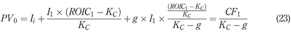
The present value of cash flow with a constant cost of capital is expressed as follows:

where PV_o is the present value of the cash flow for period 0 or the beginning of period 1, CF_i is the cash flow for period i and K_c is the cost of capital.

The above formula is applicable for multi-period cash flow. If the cash flow does not have a pattern that can be factorized, we have to estimate the cash flow for each individual period and the appropriate cost of capital. If we can predict behavior for certain periods we will be able to group the periods. For example, if we anticipate that for the first three years the cash flow of the company will grow at 10 per cent, then at 5 per cent for the next four years and thereafter at a constant perpetual growth of 3 per cent, we will have a three-stage model. On the other hand, if the cash flow grows at a constant rate from Period 1, we will have a onestage model.

If the cash flow grows at a constant rate g, it can be expressed as follows:

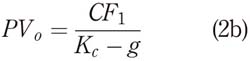
Equation (2b) is known as the constant growth one-stage model, used when the company grows at a constant rate from the outset. It is frequently used to determine the continuing value of a company of infinite life.

As we explain later, if an extraordinary return is present at the period when equation (2b) is in use, we assume these returns will remain as perpetuity for current and future investments. By "extraordinary return," we mean the return of an investment that exceeds its cost of capital. The objective of this paper is to develop a model that restricts extraordinary returns in order to present an alternative to equation (2b). We also use the expression "abnormal returns" when referring to extraordinary returns.

2.1 The dividend discount model (DDM)

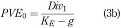
The free cash flow of a company is usually returned in the form of dividends to shareholders. Edwards and Williams (1939) present the dividend discount model:

where PVE is the present value of equity for period 0 or the beginning of period 1, Divi are the dividends of period i and KE is the constant cost of equity.

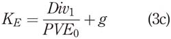
Gordon and Shapiro (1956) apply the one-stage constant growth model to dividends, assuming that they grow at a constant rate g:

In this case, KE can also be expressed as follows:

2.2 The residual income mode

An alternative to the dividend discount model is the residual income model, as found in Preinreich (1938, p. 240). The formula can be expressed as follows:

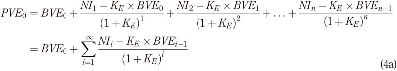
where NI_i is the net income to equity shareholders in period i, and BVEi is the book value of equity at the beginning of period i or the end of the previous period.

If the cash flow grows at a constant rate g, equation (4a) can be expressed as follows:

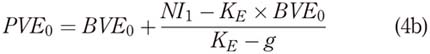
Under the assumption of clean surplus accounting, this model should yield identical results to the dividend discount model (Ohlson, 1995; Gebhardt et al., 2001; Claus and Thomas, 2001), where the difference between the net income of a company and its dividends is added to the initial book value of the period to obtain the final book value. Ohlson (1995) introduces the following equation:

where BVE_t is the book value of equity at the end of period t, BVE_t-1 is the book value of equity at the end of the previous period, NIt is the net income of period t and Divt are the dividends of period t.

Even though the dividend discount model and residual income model yield the same results, the advantage of using the residual income model is that the cash flow is estimated using the financial statements of the company. This also allows estimation of certain ratios for the forecasted period, such as net income, assets turnover, return on equity, return on capital, leverage, among other relevant ratios and their comparison with the company’s past ratios and with those of other companies in the industry. This analysis helps to adjust the model’s assumptions to achieve realistic ratios that take into account the reality of the company and industry.

2.3 The discounted cash flow model

Companies are wary of changing their dividend policy over time, as this has a signaling effect (Aharony and Itzhak, 1980). As a result of this behavior, the free cash flow to equity holders that the company generates may differ from the dividends paid. This is because firms tend to wait for earnings to stabilize before modifying their dividend policy. If the free cash flow to equity is different than the dividends paid, we can use the general discounted cash flow (DCF) model. For this purpose, we use equation (2a) and (2b). In this case, the value of the company will remain unchanged if the difference between the free cash flow to equity and the dividends is reinvested at the company’s cost of capital or distributed as stock buybacks.

Stock buybacks allow companies to distribute the free cash flow after dividends to equity holders without changing their dividend policy. Additionally, they have tax advantages when the taxes on capital gains are lower than those applied to dividend distributions.

The company value obtained by way of the DDM, the RIM and the different versions of the DCF should be the same if the assumptions are consistent and the models are correctly applied.

3. The restricted one-stage constant growth model

As noted, we call our alternative formula the restricted one-stage constant growth model. To explain it, we start with a non-growth one-stage model. We assume that new investments in fixed assets equal the depreciation and that the working capital remains constant, so in time the net investment will have a constant value and so it will be subject to zero change. Under these assumptions, the net operating profit after taxes (NOPAT) is equal to the operating cash flow in an unlevered company, where the income tax is estimated under the assumption that the company has no debt. The NOPAT is distributed as dividends, so it is also identical to the cash flow.

The present value of this company is:

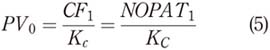
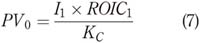
where NOPAT_i is the net operating profit after taxes for period i. The NOPAT can also be expressed in terms of initial investment and return on invested capital (ROIC):

where I_i is the invested capital at the beginning of period i and ROIC is the return on invested capital for period i. If we replace equation (6) in equation (5), we obtain the following equation:

If we subtract the initial investment from both sides of the equation, we arrive at the following equation:

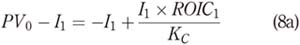
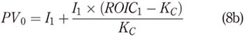
Equation (8b) allows us to separate the value into two parts: the nominal invested capital and the present value of the extraordinary return, which is equal to the difference between the return on invested capital (ROIC) and the cost of capital. The second part of the equation is the value created as a result of the difference between ROIC and KC. This extraordinary return is due to the competitive advantage of the company.

Next, we introduce a constant growth rate to our model. The company’s cash flow (or NOPAT in this case) will grow at a rate g. To achieve this growth, we have to increase our investment by g x I₁ to support the growth of future sales, and the company will have to reinvest part of its profits to support this growth. The cash flow can thus be expressed as follows:

If we insert equation (9) in equation (2b), we obtain the following:

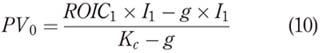
Equation (10) does not distinguish between the part of the value coming from the invested capital from the part of the value derived from future investments. To separate both values, we must use an alternative to equation (10).

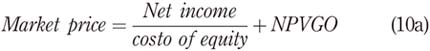
Ross et al. (2010) introduce the concept net present value of growth opportunities (NPVGO), with the following formula:

In the non-growth model, we have valued the assets in place that correspond to investments already made, so we have therefore determined the present value of these investments. However, valuing future growth concerns investments not yet made, so we must estimate the net present value of the future investments by subtracting the value of the future investment from the present value of the cash flow they will generate.

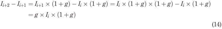
To develop the alternative equation, we start with the investment made in the first period of the perpetuity. In the period i, the company will have a new investment equivalent to the old investment multiplied by the growth rate. The new investment will be g Ii. We assume it is made at the end of period i. This new investment generates a new perpetual cash flow: NOPAT = ROIC_i g I_i. As the ROIC is assumed to be constant, ROICi can be expressed as ROIC₁.

The growth of investment made at the end of period i is as follows:

The present value of the cash flow of the investment made at the end of period i is:

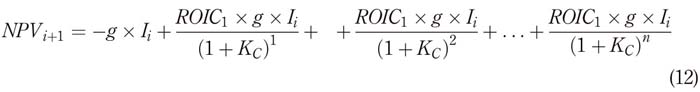
where NPV_i + 1 is the present value of the new investment made at the end of the period i. If the investment is made at the end of period i, this will be equivalent to assuming that the investment is made at the beginning of period i + 1. For example, the financial statement that closes the year (for example, that corresponding to December 31, 2017) will be the same as the one that opens the following year (the opening financial statement of January 1, 2018).

Because this is a constant in perpetuity, we can also express it as follows:

At the beginning of period i + 2 (or the end of period i + 1), a new investment is needed to support the growth. This can be expressed as:

The net present value of the new investment made at the beginning of the period i + 2 is:

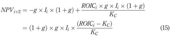
If we incorporate equation (13) into equation (15), we obtain the following result:

New investments in each of the following years will follow the same pattern. The present value of all future investments made at the beginning of each future year is:

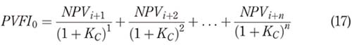
where PVFI₀ is the present value of all futures investments made after period 0. If we incorporate equation (16) into equation (17), we get the following equation:

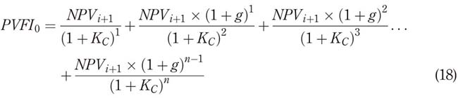
Equation (18) is a growing perpetuity that can be expressed as follows:

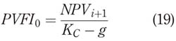
If we incorporate equation (13) into equation (19), we end up with:

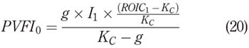
We express the present value of previous investments and the present value of future investments by adding equations (8b) and (20), to obtain the following:

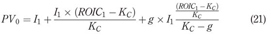
Equation (21) splits the values arising from current investments from the value that will be created by future investments. We identify three components: the current investment (i.e. assets in place); the present value of the extraordinary return over the cost of capital for previous investments; and the present value of the extraordinary return over the cost of capital of future investments. If the return on investment is lower than the cost of capital, the firm will destroy value – with negative values for the second and third item– and end up with a lower value than the amount already invested in the company.

This equation also shows that the value of a company is explained by four variables: the current investment or assets in place, the return on invested capital, the cost of capital and the growth rate.

Equation (21)shows that the relevant growth is the growth of investment. If a company reaches a certain level of stability, then sales, profits and investment will grow at a similar rate. Stability is understood to be associated with a level of efficiency that will be expressed in a constant ROIC. If there is still scope for improving efficiency, for example by selling more with the same investment level or improving the net profit with the same sales level, it will be assumed that stability has not been reached yet. Equation (21) can only be used when stability has been achieved.

If we assume that the growth rates of sales, profits and investment were different in the period of stability, we end up with absurd values. For example, if profits grow at a higher rate than investment, the long-term ROIC will be infinite. If they grow at a lower rate, it will tend to zero. If profits grow at a higher rate than sales, then in time we will end up in a position where profits are higher than sales.

In this equation, it can be easily appreciated that if the ROIC is equal to the cost of capital, then no value will have been created and the value of the company will be identical to its book value. By analyzing the growth component, we note that the growth rate is irrelevant when no value is created.

Equation (22) gives us a different cost of capital for previous investments versus future investments. If, for example, managers believe that new investments are riskier than those already made, they will be able to use a higher cost of capital for future investments to reflect this higher level of uncertainty. In this case, the equation, with a cost of capital KC1 for the current investment and a different cost of capital KC2 for future investments, is:

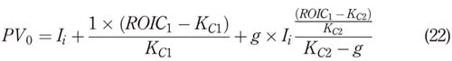
where K_C1 is the cost of capital applicable for previous investments in period I and K_C2 is the cost of capital for future investments. Equations (21) and (2b) are mathematically identical. The proof of this can be found in Appendix 1.

Equation (2b) as originally stated does not allow analysts to observe the underlying assumptions that support it. The main assumption behind this formula is that the existing competitive advantage at the period for which the continuing value is estimated will remain constant from then onwards for all investments. This holds for old and new investments alike. In the case of future investments, it assumes that the company, each year, for the rest of its life, will be able to generate new investment opportunities that will have the same competitive advantage as the previous investments, and that each of those investments will, in turn, remain for the rest of the company’s life. We have defined the extraordinary return due to competitive advantage as the difference between the ROIC and the cost of capital.

In a multi-stage model, it can be assumed that the return will equal the cost of capital in the first stages, and when this is achieved the extraordinary return will not be present in the last stage, corresponding to the continuing value. When we use a one-stage model where the extraordinary returns are present or a multi-stage model where extraordinary returns remain in the last stage, it is assumed that they will hold as perpetuity. The model we develop here is a one-stage model.

Equation (21) makes explicit the three critical assumptions embedded in the traditional unrestricted one-stage constant growth model. The first is that the competitive advantage will be perpetual for previous investments. This can be appreciated in equation (8b) in which we divide I_i x (ROIC_i- K_c) by the cost of capital K_c. Each basic point of difference between the ROIC and the cost of capital will have an impact on the value of the company.

The second assumption is that each of the new investments will also have a competitive advantage that will remain over time. This can be appreciated when in equation (13) we divide g x I_i x (ROIC_i- K_c) by the cost of capital K_c. The third assumption is that we will be able to generate new investments at a stated rate of growth g for the rest of the life of the company, each of which will generate a competitive advantage that will also remain for the rest of the life of the company. This can be seen when we divide equation (19) by ( K_C- g) .

Estimating the ROIC and comparing it with the cost of capital allows us to observe the competitive advantage being used in the valuation that constitutes the main source of value creation. This method makes the assumptions supporting the cash flow explicit, which makes evaluating their reliability possible.

Most companies tend to lose their competitive advantage over time, which is reflected in a declining ROIC that shortens the gap with the cost of capital. Conservative analysts may assume that in time the ROIC will match the cost of capital. It might also be the case that a particular company could hold a higher ROIC, which would explain a bigger gap with the cost of capital.

Knowing that the competitive advantage tends to diminish over time, we can add restrictions tob equation (21). For example, we can assume that the difference between the ROIC and the cost of capital will hold only for a period, whereas afterwards, the ROIC will be identical to the cost of capital. We can limit the number of years for which we will find new investments that will have a perpetual or limited competitive advantage. We can also use different values for the ROIC and cost of capital for previous investments versus future investments.

To limit the number of years that the competitive advantage will hold for current investments, we modify equation (8b): instead of dividing it by the cost of capital, we introduce an annuity factor. In so doing, we no longer have perpetuity, as we are substituting it for a finite horizon. We obtain equation (24):

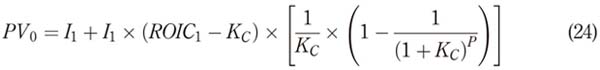
where P is the number of years in which the competitive advantage will remain for current investments.

To limit the number of years in which each of the new investments will have a competitive advantage, in equation (13), we modify the perpetuity by an annuity factor, as indicated in equation (25).

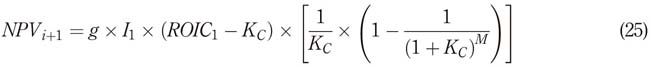
where M is the number of years each of the new investments will hold its competitive advantage.

Finally, to add a restriction to the number of years that the company will be able to generate new investments with competitive advantage, we introduce a growing annuity in equation (19). We obtain equation (26).

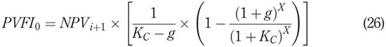
where X is the number of years that the company will be able to find new investments with competitive advantage.

If we add equation (24) and (26) and incorporate equation (25) in equation (26), we end up with the restricted one-stage growth model shown in equation (27):

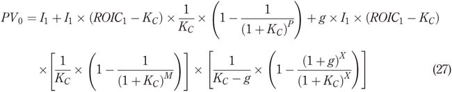
Equation (27) is the restricted one-stage constant growth model, derived from Equation (21) , which will be the unrestricted version of the model. In this equation, the restrictions will lower the ROIC in several stages until the ROIC equals KC. While in equation (21) we will have a constant ROIC as perpetuity, in equation (27) we will have a decreasing ROIC with a final value of K_C. The company will continue growing at the same constant rate in both cases, but when using equation (27), when the ROIC equals KC, the growth will be irrelevant as it will not generate value.

When indicating that the cost of capital will be set equal to the return on the investment, we have to be more specific. We can equal the ROIC to the cost of capital of an unlevered company (KU), the ROIC to the weighted average cost of capital (KWACC) or the return on equity (ROE) to the cost of equity (K_E). If we set ROIC to equal K_U we have a perpetual gap between ROIC and the weighted average cost of capital and between the ROE and the K_E. If we choose any other option, the same gap will be present in the other two alternatives.

If we equal the ROIC to K_U, we will be limiting the competitive advantage to businessrelated issues that are independent of the leverage of the company. The company will take debt if it adds value, lowering the cost of capital and increasing the gap between the return and the cost of capital.

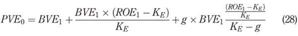
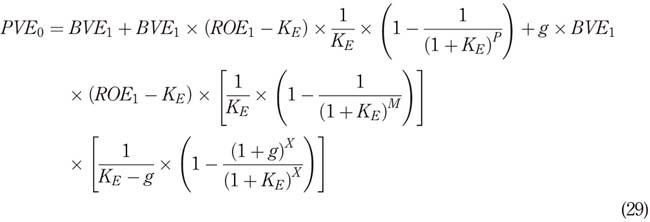
The equivalent of Equation (21) and (27) in an equity model are the following equations and (28 and and (29). They can be obtained using the same procedure.

A practical example of the application of the models is presented in Appendix 2, where use them to determine the value of the company Apple Inc.

When the new restricted values are determined through the application of and equations (27) and (29), the proportion of debt and equity of the adjusted value of capital changes with respect to the original values. This will affect the proportions of debt and equity used to determine the cost of capital. Henceforth the values of K_E and K_C will be modified, and this will require iterative solving to determine the final adjusted value of the company if we assume a constant market value debt to equity ratio.

The effect of introducing the restrictions in the model is that we assume that after a period – in this case, the higher value between P or M + X – the value of the company will equal the net value of its assets.

In the process of losing its competitive advantage, the company may be able to merge or be acquired by other companies and disappear without losing its value. In the proposed model, when the firm loses its competitive advantage and the returns equal their cost of capital, the book value of the company will be the same as the market value. The return obtained will be an adequate return under the scenario of perfect competition. In the event that the return of the company is lower than its cost of capital and there is no option to merge or be acquired by other companies, the company will have the option to continue operating with a return lower than its cost of capital, where the value will be lower than the book value, in a proportion similar to the ratio between the return and the cost of capital. If a decision is made to liquidate the company, the overestimation of its residual value will be the difference between the value obtained for its assets and its nominal value. These values that differ from the book value will be alternative options for the proposed model.

4. Conclusions

The competitive advantage of a company is reflected in the extraordinary returns over the cost of capital. Extraordinary returns attract competitors, and the greater the number of participants that enter the industry, the more pressure there is to reduce prices to a level where the returns stabilize and follow a trend toward the cost of capital.

As part of the valuation process, certain assumptions have to be made when determining the value of a company. If the company is at a stage where the return exceeds its cost of capital and this situation remains during the forecasting period, a conservative assumption will be that after a certain number of years beyond the forecasting period, the return on capital will equal the cost of capital.

The traditional one-stage constant growth formula assumes that extraordinary returns in the period in which the continuing value is estimated will remain over time as perpetuity. To correct this situation, we introduced the restricted one-stage constant growth model as an alternative to the traditional one-stage constant growth model. This facilitates observation of the competitive advantage of current and new investments embedded in the cash flow and used to estimate the continuity value.

Furthermore, the net present value from future growth is distinguished from that originating from assets in place at the moment of estimating the continuing value. The proposed formula allows the addition of restrictions to the number of years that the competitive advantage will remain for previous investments and for future investments. It also enables the limiting of the number of years that the company will be able to find new investments with the same competitive advantage. Finally, it supports the use of different returns and costs of capital for current and future investments.

The proposed model assumes that the return will equal the cost of capital when the competitive advantage disappears over a period and that the value of the company will equal its book value.

In addition to determining the continuing value of the company, the restricted one-stage constant growth model can be used to determine the impact of changing the duration of the competitive advantage in the value of the company. This sensitivity analysis will allow the analyst to determine the impact on the company’s value of variations in the duration of the extraordinary returns.

The developed model can also be used to determine the implied equity return contained in the current stock prices. If we have the information on the company’s market value, we can estimate the cost of equity that will match that value. The result will be the expected return on investing in the company. This can be estimated for individual companies and for market indexes alike.

A limitation on the application of the model is that it is necessary to assume the period in which the competitive advantage will last for the assets in place, for the number of years that the company will find new investment opportunities with positive net present values and for the number of years that the new investments will have extraordinary returns. The loss of the competitive advantage is documented in the literature, but we have not found any studies that estimate the number of years that companies can maintain their extraordinary returns. We believe that further research is needed on this subject. The model developed has the flexibility to limit the duration of the competitive advantage, but the duration of this advantage exceeds the scope of this paper and remains for future research.

A second limitation is that the return is estimated using accounting profits and registered book values, and this can vary between companies as a consequence of different accounting criteria. Two identical companies, with the same market value but different approaches to recording their operations, will have different accounting profits, registered investments, ROCI and ROE. This will create difficulties in comparing the indicators and deciding which is the correct return to apply to other companies of similar risk. To avoid such problems, analysts focus on cash flows and not accounting numbers, losing sight of the return indicators that help to determine how reasonable the assumptions of the valuation are. This limitation can be partially corrected if we adjust the company results by way of uniform accounting criteria.

The application of the restricted one-stage constant growth model to determine the continuing value of a company of indefinite life will be useful in determining a better estimate of its fundamental value.

 

References

Aharony, J. and Itzhak, S. (1980), "Quarterly dividend and earnings announcements and stockholders’ returns: an empirical analysis", The Journal of Finance, Vol. 35 No. 1, pp. 1-12.

Bhattacharya, U., Borisov, A. and Yu, X. (2015), "Firm mortality and natal financial care", Journal of Financial and Quantitative Analysis.         [ Links ]

Claus, J. and Thomas, J. (2001), "Equity premia as low as three percent? Evidence from analysts’ earnings forecasts for domestic and international stock markets", Journal of Finance, Vol. 56 No. 5, pp. 1629-1666.

Edwards, G. and Williams, J. (1939), "The theory of investment value", Journal of the American Statistical Association, Vol. 34 No. 205, p. 195.         [ Links ]

Forsyth, J. (2016), Valoracio¨n de Empresas: evitando Errores Frecuentes, Autor.

Gebhardt, W., Lee, C. and Swaminathan, B. (2001), "Toward an implied cost of capital by toward an implied cost-of-capital", Journal of Accounting Research, Vol. 39 No. 1, pp. 135-176.         [ Links ]

Gordon, M. and Shapiro, E. (1956), "Capital equipment analysis: the required rate of profit", Management Science, Vol. 3 No. 1, pp. 102-110.         [ Links ]

Inselbag, I. and Kaufold, H. (1997), "Two DCF approaches for valuing companies under alternative financing strategies (and how to choose between them)", Journal of Applied Corporate Finance, Vol. 10 No. 1, pp. 114-122.         [ Links ]

Jacobsen, R. (1988), "The persistence of abnormal returns", Strategic Management Journal, Vol. 9 No. 5, pp. 415-430.         [ Links ]

Koller, T., Goedhart, M., Wessels, D., Copeland, T. and McKinsey and Company (2010), Valuation: Measuring and Managing the Value of Companies, John Wiley and Sons.         [ Links ]

Miller, D. and Friesen, P. (1984), "A longitudinal study of the corporate life cycle", Management Science, Vol. 30 No. 10, pp. 1161-1183.         [ Links ]

Morris, J. (2009), "Life and death of businesses: a review of research on firm mortality", Journal of Business Valuation and Economic Loss Analysis, Vol. 4.
        [ Links ]
Myers, S. (1974), "Interactions of corporate financing and investment decisions – implications for capital budgeting", The Journal of Finance, Vol. 29 No. 1, pp. 1-25.
        [ Links ]
Ohlson, J. (1995), "Earnings, book value and dividends in equity valuation", Contemporary Accounting Research, Vol. 11 No. 2.         [ Links ]

Porter, M. (1998), "Competitive advantage: creating and sustaining superior performance management information systems", Vol. 19.         [ Links ]

Preinreich, G. (1938), "Annual survey of economic theory: the theory of depreciation", Econometrica (Pre-1986), Vol. 6, p. 219.
        [ Links ]
Ross, S., Westerfield, R. and Jaffe, J. (2010), Finanzas Corporativas, México.         [ Links ]

Schumpeter, J. (1942), Capitalism, Socialism, and Democracy, Harper Perennial Modern Thought.         [ Links ]

Taggart, R. (1991), "Consistent valuation and cost of capital expressions with corporate and personal taxes", Financial Management, Vol. 20 No. 3, pp. 8-20.         [ Links ]

Wiggins, R. and Ruefli, T. (2002), "Sustained competitive advantage: temporal dynamics and the incidence and persistence of superior economic performance", Organization Science, Vol. 13 No. 1, pp. 81-105.         [ Links ]

Appendix 1

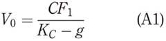
The present value of an unrestricted constant growth model can be expressed as follows:

The cash flow (CF) can be expressed as the net operating profit after taxes (NOPAT), net of reinvestment (g I1):

If we replace (A2) in (A1), we obtain the following equation:

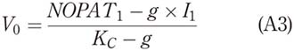
The NOPAT can also be expressed in terms of ROIC and initial investment (I_i):

If we introduce (A4) in (A3), we will obtain the following equation:

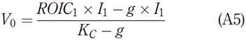
If we multiply both sides of the equation with K_c – g, we will get:

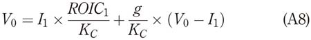
We can re express equation (A6) as follows:

Then we divide both side of the equation by K_C:

We add and subtract I1 KC KC to and from equation (A8):

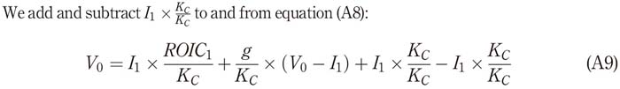
Equation (A9) can also be expressed as follows:

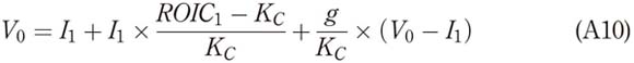
If we introduce (A3) in (A10), we will obtain the following equation:

Working on the last part of equation (A11), we obtain:

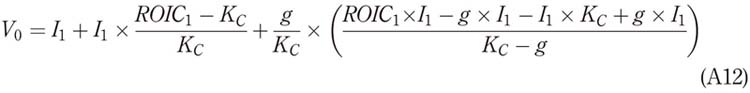
By solving equation (A12), we end up with equation (A13):

We have proved that the value of V0 of equation (A1) and (A13) are identical.

 

Appendix 2

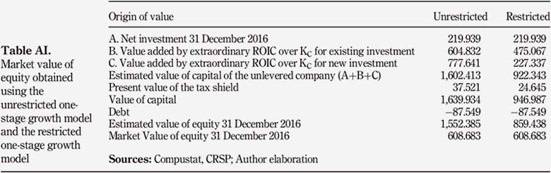
We use the company Apple Inc. to illustrate the use of equations (10), (21), (27), (28) and (29). As at 31.12.2016 the net investment of Apple was US$219.939bn, from which US$87.549bn was financed with debt and the balance of US$132.390bn by equity. We assume a ROIC of 30 per cent, a cost of capital of the unlevered company (KU) of 8.0 per cent, a cost of debt (KD) of 5 per cent and a nominal constant growth of 4.5 per cent.

We estimate the cash flow of the company using equation (9):

The present value of this cash flow is estimated using equation (10):

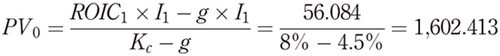
We obtain the same value with equation (21):

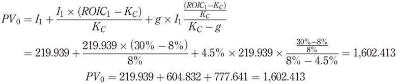
The estimated value of Apple’s capital without leverage is US$1,602.413bn. This value comes from three sources: US$219.939bn can be attributed to the capital investment; US$604.832bn to the ROIC in excess of the cost of capital for the current investment; and US$777.641bn to growth. This separation cannot be carried out using equation (2b) or its equivalent equation (10).

We can use the adjusted present value model (Myers (1974) as applied by Inselbag and Kaufold (1997) to determine the value of equity. They indicate that the value of a firm’s capital is determined by the value of the unlevered company plus the present value of the tax shield (PVTS):

We start by estimating the present value of the tax shield, which we discount using the cost of capital of the unlevered firm (KU). The tax shield for the first year is estimated by multiplying KD by the debt at the beginning of the period by the rate of corporate tax (T):

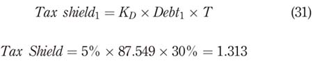
Assuming that debt also grows at 4.5 per cent, the PVTS is:

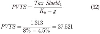
Using equation (30), we add the PVTS to the value of the unlevered company, thus obtaining the value of the capital of Apple:

To determine the value of equity we have to subtract the debt from the value of capital:

The estimated value of equity of US$1,552.385bn is much higher than the market value of equity of US$608.683bn registered on December 2016, and of US$913.220bn registered in March 2018 (at time of writing). A possible explanation of the differences in the perception of the market is that it will be difficult for Apple to sustain a ROIC of 30 per cent as perpetuity for current and future investments.

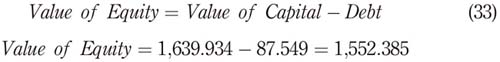
To limit the time span of the competitive advantage, we use equation (27). For this example, we assume that the ROIC for current investments will last for 20 years (P), that the company will be able to maintain the ROIC for each of the new investments (M) for 18 years, and that it will find new investment opportunities that yield the current ROIC for 15 years (X). We plug these values into equation (27):

As we are limiting the number of years in which the company will yield a competitive advantage, we also have to add limits to the number of years that the company will increase its debt. We assume that as the company is finding investment opportunities that yield a competitive advantage for the next 15 years, the debt will increase for the same 15 years at the annual rate of 4.5 per cent and then it will remain constant. With this assumption, the PVTS is reduced to 24.645 billion. The adjusted value of capital will be US$946.987bn.

By subtracting the current debt of US$87.549bn from the adjusted estimated capital value of US $946.987bn, we obtain a value of equity of 859.438 billion, which is much closer to the current market price.

In Table AI, we can appreciate the difference in value for both approaches. By restricting the time span of the competitive advantage, the value added from current investments explained by the extraordinary return over the cost of capital is reduced from US$604.832 billion to US$475.067 billion and the value added from future investments is also reduced from US$777.641 billion to US$227.337 billion.

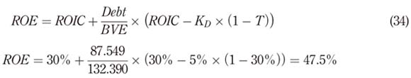
We perform the same exercise to estimate the value of the company using the equity version of the residual income model, starting off with the book value of equity. We add the assumptions that the cost of debt (K_D) is 5 per cent and that the effective corporate tax rate (T) is 30 per cent.

With this information, we estimate the ROE using the following equation:

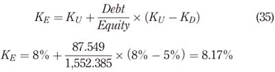
We also need to estimate the cost of equity. To do so we can use the following formula (Taggart (1991)), assuming that the tax shield is discounted with KU:

Unrestricted

Restricted

We begin by estimating the value of equity using the traditional one-stage constant growth formula found in equation (36).

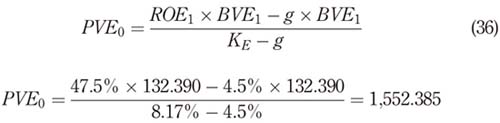
The PVE is 1,552.385 billion, which is the same equity value as that obtained in the previous valuation. To determine the origin of this value, we use equation (28):

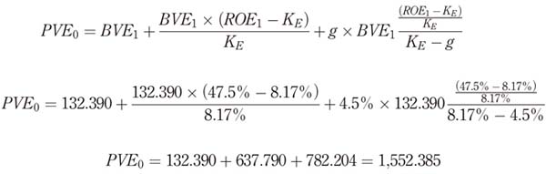
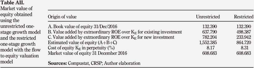
The PVE of US$1,552.385bn has the following origin: US$132.390 is the current investment, US $637.790 comes from the extraordinary return over the cost of equity for previous investments and US$782.204 comes from new investments. To limit the duration of the competitive advantage, we use equation (29) with the restricted cost of equity, as follows:

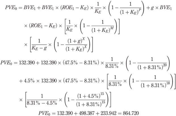
In this case, the book value of equity remains unchanged, but the value created by previous equity investments is reduced from US$637.790bn to US$498.387bn when we limit the time in which the ROE will exceed the cost of capital. The net present value of the new equity investments is reduced from US $782.204bn to US$233.942bn when limiting to 15 years the length of time in which the company will find investment opportunities that create value, and to 18 the number of years in which each of the new investments will have a ROE that exceeds its cost of capital. With these restrictions, the value of equity is reduced from US$1,552.385bn to US$864.720bn. The results are presented in Table AII.

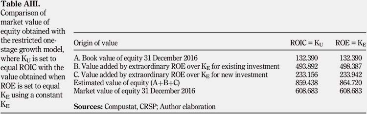
The restricted value of equity when using the equity version of the residual income model is US $864.720bn, compared to US$859.438bn obtained from the APV method. The difference is explained by:

• The gap between return and cost of capital. In the APV model, we set the ROIC to equal K_U. When doing so we observe that the K_E stabilizes at 9.77 per cent, while the ROE stabilizes at 10.98 per cent. It is impossible to close both gaps simultaneously, so when we decide to make ROIC equal to KU, we have to accept that a difference between ROE and K_E will remain in time.

• The stabilization of the cost of capital. When we add the restrictions by introducing values to the variables P, M and X, the debt to equity ratio will vary and will stabilize after the company achieves a stable ROIC. This will take place after the number of periods equal to the higher value between P + 1 and M + X + 1.

In Table AIII, we present the value of equity considering the above two points, permitting a gap between ROE and KE and the variability of the KE during the stabilization period.

 

Citation:

Forsyth, J. (2019), "An alternative formula for the constant growth model", Journal of Economics, Finance and Administrative Science, Vol. 24 No. 48, pp. 221-240. https://doi.org/10.1108/JEFAS-07-2018-0067

 

Received: 6 July 2018
Accepted: 29 October 2018