


 English (pdf)
 Article in xml format
 Article references
 Send this article by e-mail
 Cited by SciELO
  Similars in
SciELO
Similars in
SciELO 
 Permalink
1. Introduction
The literature has documented the excessive leverage utilization of inflation targeting policy instruments for growth stabilization through the call for independence of central banks. Previous studies have shown tremendous deployment and significance of inflation targeting instruments in most developing economies but without influencing their growth path (Ayres et al., 2014; Hove et al., 2017). Still, the effect of inflation targeting and its practical application as instruments was also studied to yield no-significant evidence on trade openness and financial development using a static model specification approach (Mollick et al., 2011). However, most central banks in oil-dependent developing countries were burdened with the price and financial stabilization in the mix of economic fluctuations resulted from dwelling crude-oil prices. This issue had not been given the required attention, and there was limited coverage in the literature. Hence, this study aims is to examine the optimal inflation targets for this oil-exporting Sub-Saharan African (SSA) countries over the period 1996-2017.
It is worthy to note that optimal inflation targeting could help most central banks in this region to formulate appropriate monetary policy and use this preventive measure. Likewise, policymakers might need to coordinate monetary and exchange rate policy in the efficacy of alternative methods of targeting the exchange rate as envisaged in Buffie et al. (2018). This is the contribution of the study to the literature by providing a shred of evidence from a dynamic heterogeneous panel threshold model for 15 major oil-exporting SSA countries.
Furthermore, the previous study’s methods were studies that used linear models to investigate the relationship between inflation and exchange rate, which produced mixed conclusions regarding the relationship between exchange rate and inflation-growth nexus. Abo-Zaid and Tuzemen (2012) investigated the effect of inflation targeting on growth and fiscal imbalances in most inflation targeting developing countries showing stable economic growth than the non-targeting countries. Ambaw and Sim (2018) investigated the effectiveness of inflation targeting instruments on a fixed exchange rate regime to attract FDI inflows in developing countries using propensity score matching methodology, and their findings revealed that there was no significant evidence for the policy instrument to attract FDI. Similarly, there is no consensus about a steady-state of the relationship among studies (Abbott et al., 2012; Abo-Zaid and Tuzemen, 2012; Gonçalves and Salles, 2008; Huang et al., 2009; Lin and Ye, 2012; Siklos, 2007).
Therefore, it is praiseworthy to apply a non-linear panel threshold model developed by Hansen (2000) to investigate the relationships between inflation targeting and real exchange rate (RER). This requires an examination of the optimal inflation targets in this sample of 15 major oil-exporting SSA countries. The application of a pooled panel sample becomes essential as this approach improves the statistical efficiency and power of the empirical estimation. Consequently, it dampens the parameter estimates bias associated with the sample period and the homogeneity of the cross-sectional entities.
To achieve this, we apply Hansen’s panel threshold technique to explore the relationship between inflation threshold-effect and RER. The estimation technique is significant in exploring the threshold level of inflation rather than using a technique that does not embed a split-sample approach. There are previous studies that applied non-linear threshold techniques on the inflation regime and they are Aleem and Lahiani (2014), Baharumshah et al. (2016) and Yi and Xiao-li (2018).
There are limited studies in the literature that focused on optimal inflation targets for oil- exporting SSA countries. Based on this study panel data from 15 major oil-exporting SSA countries, namely, Angola, Cameroon, Chad, Congo Rep, Congo DPR, Cote d’Ivoire, Equatorial Guinea, Gabon Ghana, Malawi, Niger, Nigeria, South Africa, Sudan and Zambia.
Our results revealed evidence of threshold inflation targets of 14.47 per cent for these countries. Therefore, this indicates that raising inflation level beyond the threshold level will adversely affect the monetary policy agenda and the exchange rate policy. The rest of the paper is structured as follows. Section 2 presents the literature on inflation targeting and exchange rate. Section 3 presents the method and data analysis. Section 4 presents the interpretations of estimations and tests. Finally, Section 5 concludes the paper.
2. Review of the literature
Several empirical studies have focused on inflation targeting as a policy tool in the conduct of monetary policy. Monetary policy has different perspectives towards approaching inflation targeting but best among those perspective is the evaluation of exchange-rate policy (Chang and Velasco, 2000). Inflation targeting as a policy tool was sustainable given the conditions of prudence and accountability of the central bank, and it was achieved under ideal central bank independence (Svensson, 2010). Aizenman et al. (2011) investigated the role of the RER and inflation on commodity and non-commodity as a mixed strategy for interest rate policy in emerging market economies. Their findings revealed a significant impact on the RER for the countries that adopted inflation targeting policy relative to the countries with non-inflation targeting regime. Hughes Hallett and Proske (2017) investigated the relationships between inflation regimes under the conditions of projected volatility and income growth in OECD and developing countries using Rogoff (1985) model. Their findings revealed a significant impact of central banking conservatism in stabilizing the economic growth in the OECD countries. Caporale et al. (2018) investigated the efficacy of monetary policy framework on the perspective of Taylor’s rule in five emerging market economies, namely, Turkey, Thailand, South Korea, Israel and Indonesia using non-linear threshold technique[1]. Their findings revealed the reaction of the central banks towards deviation from targeting using either inflation framework or output targets as motivated by the significance of the estimate from the sampled countries given the conditions of a low or high inflation regime. Furthermore, the result suggests that the exchange rate impact was significant to the inflation targeting regime.
Some of the prior studies uncovered the effectiveness of inflation targeting monetary instrument in converting the menace of price fluctuations resulting from macroeconomic instability towards the adoption of inflation targeting framework as a monetary policy tool for most of the central banks in developing countries and emerging market economies. This study would constraint the review of existing literature to emerging markets economies than on African countries as only South Africa and Ghana had officially announced adopting inflation targeting as a tool for monetary policy (Umar and Dahalan, 2017). According to Kasekende and Brownbridge (2011), monetary framework that used inflation targeting is not appropriate for SSA countries, even though it proved usefulness in damping inflation. However, Siregar and Goo (2010) investigated the effectiveness of inflation targeting framework and its validity in damping the shocks in output and inflation risk for Thailand and Indonesia. In another related study, Prasertnukul et al. (2010) uncovered the usefulness of inflation targeting framework in Asian countries. Their findings revealed that the framework practicality reduced exchange rate pass-through in Thailand and South Korean, while indifferent for the Philippines and Indonesia. Furthermore, many other studies also showed that inflation targeting framework is most effective in financial and banking sector stability (Fazio et al., 2015; Tabak et al., 2016; Ismailov et al., 2016; Soe and Kakinaka, 2018; Cornand and M’Baye, 2018). Nevertheless, some studies reported on the efficacy of the inflation targeting framework in exchange rate policy as in Khodeir (2012), who explored the flexible targeting regime for Egypt. Yamada (2013) discovered inflation targeting worked for a fixed regime than the flexible regime in the case of developing countries, his result corroborated with the findings from Umar and Dahalan, (2017).
In most recent studies, Taylor (2019) uncovered the link between monetary policy and inflation targeting. He suggested that targeting inflation alone cannot be achieved without monetary policy rule and vice versa. Coulibaly and Kempf (2019) explored the inflation targeting framework effectiveness and whether the framework would be efficient in damping inflationary environment for merging market economies. Their findings revealed that the inflation targeting framework was favourable to forward bias through fading uncovered interest rate parity conditions. They also reported that inflation targeting promotes stability in financial sectors. A review from inflation targeting open economies, Makin (2019) revealed that appropriate policy on inward strategy for productivity enhancement tends to control the pressure of inflation and price level in the medium term. On the Brazilian economy, Díaz-Roldán et al. (2019) affirmed that fiscal rules and fiscal discipline under inflation targeting regime help in controlling the inflationary environment in Brazil. More so, Okimoto (2019) acknowledged that there was a strong link between inflation regime and monetary policy regime in Japan using smooth transaction Phillip curve model. His findings revealed that qualitative and quantitative easing were the solutions for the escaped deflationary regime in Japan.
Contrary to the above, Fukuda and Soma (2019) discovered that the Bank of Japan subscribed to explicit inflation targeting framework, and the framework was not effective in inflation targeting regime. In the same vein, in the case of India, Mohan and Ray (2019) reviewed the effectiveness of monetary policy and inflation targeting in the case of deteriorating Indians public sector expenditure during demonetization episode. Their findings revealed that the Indian monetary policy was more effective. Koirala et al. (2019) explored three policy rules as real sector required some degrees of external credit. Their finding revealed that for the three policies, namely, inflation targeting framework, Taylor’s rule and unemployment rule, only monetary policy for unemployment was able to combat most macroeconomic fluctuations. Bonga-Bonga and Lebese (2019) examined a stable inflationary environment corresponding to the level of unemployment in South Africa. They used the non-accelerated inflation rate of unemployment to explore the time-varying Phillips curve model. Their findings revealed that inflation targeting does not work for the South African economy as Phillip curve turned vertical. Therefore, the consensus about usefulness of inflation targeting in financial stability and central bank autonomy have been mixed.
It was because of the gap in the literature that this study intended to establish an optimal inflation target for 15 major oil-exporting SSA countries, a question raised by Bonga-Bonga and Lebese (2019) as to whether 3-6 per cent was an optimal inflation band for South Africa? As there is no consensus in the literature regarding the optimal inflation targeting in the emerging markets, it has motivated us to undertake the study on selected SSA countries. This study used a dynamic panel threshold technique to assess whether there are optimal inflation targets, which point to threshold-effect and an asymmetrical relationship between inflation and the RER may exist.
3. Data and methodology
This study follows the approach by Ahmad and Abdullah (2013) and Umar and Dahalan (2017) to inflation targeting framework and augmented with the RER and consumer price on panel threshold regressive model developed by Hansen (1996, 1999, 2000). The panel cointegration test is performed after confirming that all the variables are stationary. The panel threshold model can be written as follows:
where OIit represents the optimal inflation, which is measured by inflation rate dit (inflation) is the explanatory variables and also the threshold variable. There are four control variables fit, which may affect the exchange rate. Ø 1, Ø 2, Ø 3 and Ø 4 represent the heterogeneity of the countries under heterogeneous operating conditions; is the threshold coefficient when the threshold value is lower than is the threshold coefficient when the threshold value is higher than g , the errors ɛit are assumed ; i represents heterogeneous countries (entity) and t represents the years.
This approach used an augmented Hansen (1999) and Caner and Hansen (2004) that uses the simulation likelihood ratio to test the asymptotic distribution of threshold estimate using two-stage ordinary least squares method via minimizing sum of squared of errors, S1(y ) where threshold value Ŷ and residual variance σ2 can be obtained. The null hypothesis of no threshold effect H0 = = is tested against the alternative hypothesis, using likelihood ratio test where , and S0, S1 (Ŷ) are the sum of squared errors. Notwithstanding, the bootstrapping procedure would produce the p-values and critical values that are asymptotically proven. This would reveal the threshold-effect between inflation and the RER. Thus, the asymptotic distribution of the threshold estimate is tested with the null hypothesis, H0 = y = y0 , using the likelihood ratio statistics test of . The asymptotic confidence interval is shown as where for a given asymptotic level , the null hypothesis of y = y0 is rejected if LR1(y ) is above c ( ).
Furthermore, the model is modified if a double threshold exists. It can be shown as follows:
where the threshold value is y1 < y2 . The model can be extended to multiple thresholds using a similar approach.
The annual data for consumer price index (CPI); inflation rate, trade openness (OPEN) are sourced from World Bank Development Indicators (WDI) (2018), while RER is calculated by multiplying the nominal exchange rate by the relative ratio of the CPI, and squared terms series are generated using Stata 14 statistical software.
4. Empirical results
The empirical results start with the reported results from panel unit root tests and confirm that the variables are stationary at I (0). Table 1 presents the panel unit root tests for Hadri, ADF-Fisher and PP-Fisher (Hadri, 2000; Choi, 2001; Maddala and Wu, 1999). The tests revealed that all the variables are stationary as the null hypothesis for the unit root is rejected.
Table 2 presents the results of cointegration tests of the individual-specific effects with structural break analysis following an approach proposed by Gregory and Hansen (1996) test using ARDL-ECM framework. According to Gregory and Hansen (1996), once break v is evident in a data such that if it is ignored and simply estimates the regression, the result may lead to wrong inferences, which are not best for the model. The break dates v denoted by higher negative values of ADF, Zt and Za through comparing to the least result for the null hypothesis. If Zt statistics is significant, reject the null hypothesis. The structural breaks test is conducted with constant, constant and break, and slope, respectively.
From Table 2, both ADF and Zt statistics are assumed to be higher than 5 per cent asymptotic critical values. The rule of thumb is that the lower the statistics value the better the model. On the panels, we have countries with significant break years and some with nosignificant breakpoints. Countries with significant break year include Angola in 2014, Nigeria in 2010, Sudan in 2011 and Zambia in 2013. On the other hand, countries without significant breakpoint are Cameroon, Chad, Congo Democratic Republic, Congo Republic, Cote d’Ivoire, Equatorial Guinea, Gabon, Ghana, Malawi, Niger Republic and South Africa. Therefore, our data were having significant break years of 2010, 2011, 2013 and 2014[2]. Next, we included dummy variables to capture the structural break in the model.
Table 3 presents the robustness analysis using auxiliary traditional panel regression analysis. The results present the robustness of the regressions using three models, the first model estimation without dummies (Columns 2-3), the second model estimation with dummies (Columns 4-5) and the third model estimation excludes the outliers (Columns 6-7). The essence is to explore how robust outliers detection proposed by Cook (1977, 1979) distance measure, and structural dummy affected the empirical results.
In Table 3 (Columns 2-3) presents the random and fixed effect models estimates without consideration of structural break in the data. The results from random and fixed effect models revealed only consumer price variable is statistically significant at 1 per cent. In Columns 4-5, when the structural dummy is factored in the models the results drastically changed. The significant structural dummy improved the estimates for the better, revealed that consumer price and trade openness enters 1 per cent statistically significant levels. However, the results manifested that a structural break dummy has great influence in our models. Similarly, when compared with exclusion of influential data points (outliers) in the models in Columns 6-7, even though not much variation with the models with break dummy but revealed the best estimates compared to earlier models without structural break. Hence, outliers drastically influenced our empirical estimates as all the coefficients of consumer price, trade openness and inflation appeared statistically significant at 5 per cent levels. Hence, the models are well specified through the heteroskedasticity and Breusch-Pagan LM tests.
Table 1
.| Regressors | Hadri | ADF-Fisher | PP-Fisher | |||
| RER | 7.72312*** | 55.0418*** | 65.2764*** | |||
| CPI | 4.70768*** | 49.0189** | 101.807*** | |||
| Squared RER | 7.56267*** | 54.9035*** | 63.7218*** | |||
| Squared CPI Inflation rate | 5.60135*** | 5.51868*** | 42.9787** | 190.702*** | 80.8545*** | 1218.07*** |
| OPEN | 15.4072*** | 125.698*** | 296.256*** | |||
| Notes: ***; **; *designating statistical significance at 1, 5 and 10%, respectively, for rejecting the null hypothesis for the presence of unit root | ||||||
| Source: Author’s compilations | ||||||
Table 2
.| ADF | Zt | Za | |||||
|---|---|---|---|---|---|---|---|
| Panels | Gregory and Hansen models | Statistics | Break point | Statistics | Break point | Statistics | Break point |
| Angola | Change in level | -3.07 | 2014 | -3.22 | 2014 | -17.25 | 2014 |
| Change in level with trend | -6.08** | 2013 | -7.53** | 2014 | -32.44 | 2014 | |
| Change in regime | -6.05** | 2010 | -3.59 | 2011 | -16.25 | 2011 | |
| Cameroon | Change in level | -3.71 | 2003 | -3.90 | 2003 | -16.29 | 2003 |
| Change in level with trend | -4.78 | 2003 | -4.90 | 2003 | -21.55 | 2003 | |
| Change in regime | -4.09 | 2002 | -4.19 | 2002 | -20.21 | 2002 | |
| Chad | Change in level | -4.27 | 2001 | -4.37 | 2001 | -20.11 | 2001 |
| Change in level with trend | -4.21 | 2001 | -4.32 | 2001 | -19.78 | 2001 | |
| Change in regime | -4.38 | 2001 | -4.48 | 2001 | -21.21 | 2001 | |
| Congo Dem. Rep | Change in level | -3.53 | 2010 | -3.43 | 2009 | -16.69 | 2009 |
| Change in level with trend | -4.11 | 2009 | -4.21 | 2009 | -20.14 | 2009 | |
| Change in regime | -5.28 | 2008 | -5.41 | 2008 | -25.62 | 2008 | |
| Congo Republic | Change in level | -4.16 | 2004 | -3.31 | 2004 | -15.13 | 2004 |
| Change in level with trend | -4.16 | 2004 | -3.84 | 1998 | -18.20 | 1998 | |
| Change in regime | -4.18 | 2004 | -4.28 | 2004 | -19.76 | 2004 | |
| Cote d’Ivoire | Change in level | -4.27 | 1998 | -4.51 | 1998 | -20.37 | 1998 |
| Change in level with trend | -4.17 | 1998 | -4.42 | 1998 | -19.97 | 1998 | |
| Change in regime | -5.06 | 2002 | -5.18 | 2002 | -24.16 | 2002 | |
| Equatorial Guinea | Change in level | -3.99 | 1999 | -4.44 | 1999 | -19.89 | 1999 |
| Change in level with trend | -4.73 | 2004 | -4.28 | 1999 | -19.86 | 1999 | |
| Change in regime | -4.12 | 2004 | -4.22 | 2004 | -19.52 | 2004 | |
| Gabon | Change in level | -3.96 | 2003 | -4.24 | 2003 | -18.75 | 2003 |
| Change in level with trend | -5.13 | 2002 | -5.26 | 2003 | -20.71 | 2003 | |
| Change in regime | -4.35 | 2004 | -4.68 | 2004 | -17.51 | 2004 | |
| Ghana | Change in level | -2.84 | 2005 | -4.01 | 2014 | -22.19 | 2003 |
| Change in level with trend | -4.40 | 2008 | -4.51 | 2008 | -21.57 | 2008 | |
| Change in regime | -4.01 | 2008 | -4.11 | 2008 | -19.64 | 2008 | |
| Malawi | Change in level | -3.05 | 2009 | -4.02 | 2014 | -21.04 | 2014 |
| Change in level with trend | -5.08 | 2012 | -6.42 | 2012 | -28.82 | 2012 | |
| Change in regime | -4.88 | 2011 | -4.49 | 2008 | -21.72 | 2008 | |
| Niger Republic | Change in level | -4.34 | 2004 | -4.20 | 2003 | -18.42 | 2003 |
| Change in level with trend | -4.53 | 2003 | -4.65 | 2003 | -19.71 | 2003 | |
| Change in regime | -4.24 | 2004 | -4.25 | 2002 | -19.58 | 2002 | |
| Nigeria | Change in leve | -3.65 | 2006 | -2.76 | 2014 | -16.20 | 2014 |
| Change in level with trend | -4.51 | 2000 | -2.96 | 1999 | -12.92 | 1999 | |
| Change in regime | -7.11** | 2010 | -3.86 | 2010 | -20.37 | 2010 | |
| South Africa | Change in level | -3.38 | 2007 | -3.47 | 2007 | -16.55 | 2007 |
| Change in level with trend | -4.19 | 2009 | -3.66 | 2009 | -17.92 | 2009 | |
| Change in regime | -4.29 | 2007 | -3.50 | 2013 | -16.80 | 2013 | |
| Sudan | Change in level | -11.19** | 2012 | -10.26** | 2014 | -42.34 | 2014 |
| Change in level with trend | -6.98** | 2012 | -9.14** | 2014 | -43.37 | 2014 | |
| Change in regime | -7.27** | 2012 | -6.98** | 2011 | -37.41 | 2011 | |
| Zambia | Change in level | -4.75 | 2014 | -4.87 | 2014 | -22.68 | 2014 |
| Change in level with trend | -4.49 | 2014 | -4.63 | 2014 | -20.23 | 2014 | |
| Change in regime | -6.40** | 2007 | -5.74** | 2013 | -29.23 | 2013 | |
| Note: **Denotes significance at 5% level. The 5% critical values for ADF (and Zt) are -4.92, -5.29 and -5.50 for Models 1, 2 and 3, respectively, while the Za for the same models are -46.98, -53.92 and -58.33, respectively. Stata commands Gregory and Hansen (1996) “ghansen” is used with optimal lag structure chosen by the Bayesian information criterion | |||||||
| Source: Authors’ computations | |||||||
Table 3
.| RE model without | ||||||
| break | FE model without | RE model with | FE model with | RE model | FE model excludes | |
| Variable | dummies | break dummies | break dummies | break dummies | excludes outliers | outliers |
| Constant | 63.16 (69.54) | 66.20** (29.57) | 72.60 (54.90) | 83.16*** (22.15) | 150.1*** (43.04) | 165.4*** (21.60) |
| CPI | 2.688*** (0.198) | 2.685*** (0.199) | 1.057*** (0.178) | 1.070*** (0.179) | 0.536*** (0.167) | 0.551*** (0.165) |
| OPEN | 0.293 (0.246) | 0.258 (0.251) | 0.523*** (0.183) | 0.501*** (0.187) | 0.421** (0.164) | 0.381** (0.165) |
| Inflation rate | 0.0115 (0.0449) | 0.0121 (0.0451) | -2.56e-05 (0.0333) | 0.000927 (0.0335) | -0.869*** (0.189) | -0.852*** (0.186) |
| ydum1 | 0.476*** (0.0386) | 0.469*** (0.0389) | 0.420*** (0.0347) | 0.410*** (0.0343) | ||
| ydum2 | 0.165*** (0.0476) | 0.166*** (0.0479) | 0.171*** (0.0468) | 0.172*** (0.0462) | ||
| ydum3 | -0.174* (0.101) | -0.178* (0.101) | -0.143 (0.0878) | -0.147* (0.0863) | ||
| ydum4 | 131.3 (196.9) | _ | 238.7 (147.3) | _ | ||
| Breusch-Pagan LM test p- value | 0.0000 | 0.0000 | 0.0000 | |||
| Heteroskedasticity p-value | 0.0000 | 0.0000 | 0.0000 | |||
| Hausman test p-value | 0.8552 | 0.9136 | 0.4578 | |||
| Number of code | 15 | 15 | 15 | 15 | 15 | 15 |
| Observations | 330 | 15 | 330 | 330 | 313 | 313 |
| R2 | 0.374 | 0.659 | 0.612 | |||
| Notes: Standard errors are in parentheses; ***; **; *denoted 10, 5 and 1 pet cent, statistically significant levels, respectively. ydum = year dummy | ||||||
| Source: Author’s compilations | ||||||
Departing from the linear model specification, we used nonlinear panel dynamic threshold model specification proposed by Hansen (2000) and Caner and Hansen (2004). The estimation procedure begins with a threshold-effect test, the results are presented in Table 4 [3].
Table 4 presents the threshold-effect test with a structural dummy. The F-statistics test for the triple, double and single thresholds effect comprising their bootstrap p-values. The study used 1,000 replications for each of the mentioned bootstrapping procedure tests. The F-statistics test result shows that the single threshold is 11.90 and was statistically significant at the 5 per cent level, as it is above the critical value of 9.39. Nevertheless, the tests for the triple and double threshold effects were not significant with their bootstrapping p-values of 0.505 and 0.980, respectively. Therefore, the study concludes that there is overwhelming evidence of a single threshold effect of inflation on RER for major oilexporting SSA countries.
Henceforward, this study concentrates on the single threshold model. The finding from the above also shown that the estimated value for the single threshold was found to be 14.47 per cent thus splitting all observations into two regimes. Table 5 reports the estimated coefficient based on OLS standard errors and their p-values. The result revealed that inflation has a negative and statistically significant effect in terms of trade and the squared consumer price value.
It is worth note, the primary concern is those coefficients and by each of the regimes. The estimated coefficient of the first regime is (-3.147), which is significant at 1 per cent level.
Table 4.Results
| Threshold variable: inflation | Result | |
|---|---|---|
| Test for single threshold | ||
| 14.47 | ||
| F1 | 11.90 | |
| p-value | 0.020** | |
| (10, 5 and 1% critical values) | (7.63, 9.39 and 13.24) | |
| Test for double threshold | ||
| 14.47 | ||
| 4.37 | ||
| F2 | 3.10 | |
| p-values | 0.5050 | |
| (10, 5 and 1% critical values) | (8.72, 10.27 and 13.84) | |
| Test for triple threshold | ||
| 14.47 | ||
| 4.37 | ||
| 3.01 | ||
| F3 | 0.88 | |
| p-values | 0.9800 | |
| (10, 5 and 1% critical values) | (11.92, 14.44 and 18.36) | |
| Notes: Significant at: ***; ;** and *designating 1, 5 and 10 %, respectively. F-statistics and p-values are from the bootstrap procedure 1,000 times for each of the three bootstrap tests | ||
| Source: Author’s compilations | ||
This implies that inflation decreases by 3.147 per cent with a decrease of 1 per cent inflation rate for major oil-exporting SSA countries that have an inflation rate of less than or equal to 14.47 per cent. In the second regime, if the inflation rate is above 14.47 per cent, the estimated coefficient is (-0.0022). However, it is not significant, which indirectly referred to as; there is no impact of inflation on RER when that inflation rate is above 14.47 per cent. The result was spontaneous, suggests that an increase in inflation rate beyond a certain threshold level of 14.47 per cent would have no impact on the RER and would just consider depending on the countries level of leverage.
The control variables in the model also shown that an annual variation in squared RER, and squared CPI, excluding trade openness, are statistically significant in explaining the impact of RER and inflation rate. Both squared terms are significant at 1 per cent affirmed that there is a certain limit for which the impact of the variables of interest can explain variations on one another. This indicates that the lesser terms of trade, and that of both squared terms, the higher the RER. The estimated coefficients of terms of trade and consumer price are -8.942 and 2.826, respectively. Even though, the trade openness variable shows that it positively explains RER but lost significance from the OLS standard errors and p-value.
Figures 1 shows the graph depicting optimal inflation targets for 15 major oil- exporting SSA countries over the period 1996-2017. The LR function diagram of the single threshold model is used to investigate the consistency of the true threshold and the estimated threshold value to give a better picture of the accuracy of the threshold estimates and the confidence intervals. The inflation threshold level is the threshold estimation value when the long-run ratio LR value is zero. The graphs presented in Figures 1 are for the first and second threshold parameters of the inflation threshold levels for 14.47 and 4.37, respectively when the LR value is zero. The confidence interval of the threshold estimation value is the interval of the inflation threshold level, that approximate to less than the long-run ratio LR = 7.3523, with the confidence interval at 95 per cent. Consequently, the confidence interval of threshold estimation values 14.47 and 4.37 are [7.63 - 13.24] and [8.72 - 13.84], respectively. As the corresponding confidence interval contains two threshold estimation values, the threshold estimation value is consistent with the true threshold value.
Table 5
.| Regressor RER | Coefficient | S. E | t | p > |t] |
|---|---|---|---|---|
| CPI | 2.826 | 0.212 | 13.33 | 0.000 |
| OPEN | _0.0148 | 0.0958 | _0.15 | 0.877 |
| Squared RER | 0.000560 | 1.85e_05 | 30.28 | 0.000 |
| Squared CPI | -0.00817 | 0.000822 | _9.93 | 0.000 |
| SB Dummy1 | 0.0542 | 0.0239 | 2.27 | 0.024 |
| SB Dummy2 | -0.155 | 0.0283 | _5.49 | 0.000 |
| y 1 ≤ 14.47% | _3.147 | 0.975 | _3.23 | 0.001 |
| y 2 > 14.47% | _0.00220 | 0.0172 | -0.13 | 0.898 |
| Note: RER = real exchange rat | ||||
| Source: Author’s compilations | ||||
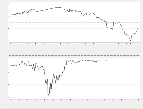

Figure 1
.5. Conclusions
This study investigates the optimal inflation targets in a panel of 15 major oil-exporting SSA countries using annual data over the period 1996-2017. It used a threshold panel model to examine the threshold-effect test and threshold estimation following the ordinary least squares likelihood ratio developed by Hansen (1999). The threshold-effect test revealed a single threshold level of 14.47 per cent. The findings allow the policymakers in the region to leverage on these important findings, and an inappropriate decision might have serious implications in the monetary policy rule.
Furthermore, the study response to the question of whether an appropriate inflation targeting influences the RER or whether there is an optimal inflation level at which these countries could appropriately maximize leverage on foreign exchange potentials. The study also provides new sight on the existence of a threshold inflation target of 14.47 per cent for these countries. Other variables that can still explain the relationship between inflation regime and the RER in the model are consumer prices and trade openness. The impact of consumer prices was positively significant while the impact of trade openness was negative and not significant. Further studies need to be carried out to unveil the overpowering impact of trade openness in a model of inflation target regimes.
The policy implications of these findings insinuate that the inflation target rate below the threshold value is appropriate and in line with prior expectations. Keeping inflation low in a low-inflation environment is preferred than getting inflation down from above threshold value of 14.47 in a high-inflation regime as envisaged in (Taylor, 2019).
Notes
1. See Taylor (2000).
2. The output of the regression is available upon request.
3. In this model, the threshold-effect test was conducted using a structural break dummy. Further, an auxiliary threshold-effect test was also conducted without break dummy for robustness analysis. The result revealed that F-statistics of the auxiliary regression for the single threshold is 10.66 and was statistically significant at the 10 per cent level. Nevertheless, the auxiliary regressions for the triple and double threshold-effects were not significant with their bootstrapping p-values of 0.964 and 0.276, respectively.

