


 English (pdf)
 Article in xml format
 Article references
 Send this article by e-mail
 Cited by SciELO
  Similars in
SciELO
Similars in
SciELO 
 Permalink
1. Introduction
There is widespread argument that well-developed financial markets play a key role in promoting economic growth (see, for instance, Adeniyi et al., 2015; Capasso, 2008; Jedidia et al., 2014; Levine, 1997; Otchere et al., 2016; Pradhan et al., 2015; Uddin et al., 2013; Wachtel, 2001). The importance of the relationship between the development of financial markets and economic growth is well recognized throughout the financial literature (Bhattarai, 2015; Greenwood and Scharfstein, 2013; Iyare and Moore, 2011; Peia and Roszbach, 2015; Samargandi et al., 2015). Theoretically, financial development[1] contributes to economic growth through a variety of channels, such as ameliorating risk, reducing information asymmetries, monitoring enterprises and promoting corporate governance, liberalizing the exchange of goods and services and mobilizing savings (Pradhan et al., 2017a; Ngare et al., 2014; Owusu and Odhiambo, 2014; Thumrongvit et al., 2013; Hsueh et al., 2013; Zhang et al., 2012; Levine, 2005; Levine, 2003; Levine et al., 2000; King and Levine, 1993a, 1993b). Several studies[2] provide supporting evidence that financial development contributes to economic growth (see, for instance, Pradhan et al., 2014a, 2014b, 2014c). However, many of these studies focus on the overall development of financial markets with little to no attention being given to the development of either stock markets or bond markets[3]. Moreover, the research on the relationships between bond market development and economic growth is scarce in the growth and financial literature alike (Egert, 2015; Mu et al., 2013; Sharma, 2001).
It can be noted that both stock market development and bond market development have links to economic growth through a variety of sub-connections (Bui et al., 2018; Benczúr et al., 2018; Pradhan et al., 2016a, 2016b; Peregoa and Vermeulena, 2016; Mu et al., 2013; Thumrongvit et al., 2013; Bhattacharyay, 2013; Sophastienphong et al., 2008). Furthermore, the stock market and bond market developments also correlate with each other (Kourtellos et al., 2013; Checherita-Westphal and Rother, 2012; Fink et al., 2003; Rahman and Mustafa, 1997). Evidently, there is no shortage of research on the links between stock and bond market development and economic growth. While the direction of Granger causality between economic growth and these variables is not always uniform across studies, the weight of the evidence supports the notion that both stock and bond market development positively impact economic growth. At the same time, an under-researched area is the link between stock market development and bond market development itself. In this paper, we focus on the inter-links between all of these variables. In addition, we examine the nature of causality in the presence of two additional key macroeconomic variables, namely inflation rate and real interest rate bringing our full set of variables to five. The empirical question is whether there is Granger causality[4] among these five variables.
Having a better understanding of the dynamics between stock market development and bond market development and their simultaneous connection to economic growth and other macroeconomic variables offers important lessons for policymakers. For instance, our study asks whether the co-development of the stock market and bond market is necessary for economic growth and whether feedback causality exists (i.e. whether causality flows in the opposite direction as well). Moreover, we report on both short- and long-run causality among the variables.
The remainder of this paper is organized as follows. Section 2 presents the theoretical framework. Section 3 presents a review of the literature. Section 4 describes our data, variables, and model. Section 5 describes our econometric methodology. Section 6 presents and discusses the results. Section 7 concludes with policy implications.
2. Theoretical framework
It is a well-established fact that long-run economic growth solely depends on the ability to increase the speed of the accumulation of physical and human capital, to use the resulting productive assets more efficiently and to guarantee access of the whole population to these assets. Financial intermediation provides this investment process by mobilizing savings for investment by firms:
ensuring that these funds are allocated to the most productive use; and
spreading risk and providing liquidity so that the firms can operate the innovativecapacity efficiently.
Therefore, financial development involves the formation and development of institutions, instruments, and markets that support this investment process and to achieve economic growth. Usually, the role of banks and non-bank financial intermediaries, ranging from pension funds to stock markets, has been to translate household savings into enterprise investment, monitor investments and allocate funds, and to price and spread risk. Yet financial intermediation has strong externalities in this context, which are generally positive, such as information and liquidity provision, but can also be negative in the systematic financial crises which are endemic to market systems. Financial development and economic growth are thus clearly related, and this relationship has occupied the minds of great economists such as Robinson, Schumpeter and Goldsmith (Levine et al., 2000; Levine, 1997).
In the development literature, the financial system is the nerve center of a country’s development. Hence, an efficient provision of financial services determines the economic growth and prosperity of a country (see, for instance, Pradhan et al., 2017a, 2017b). Financial development can contribute to economic growth in the following ways:
ensuring financial stability;
supporting trade and commerce;
mobilizing domestic savings;
allowing different risks to be managed more recently by encouraging the accumulation of new capital;
increasing a more efficient allocation of domestic capital; and
aiding to reduce or mitigate losses.
Historically, the role of financial development on economic growth has received considerable attention since the emergence of endogenous growth theory. The theoretical contributions on this area can be divided into various strands. First, the allocative role of financial systems (Greenwood and Jovanovic, 1990). Second, financial markets allow firms to diversify portfolios, to increase liquidity, which reduces risks, and hence stimulates growth (Levine, 1997). Third, financial development provides an exit mechanism for agents and improves the efficiency of financial intermediation (Arestis et al., 2001). Fourth, the financial market’s ability to impact economic growth through changes in incentives for corporate control (see, for instance, Demirguc-Kunt and Levine, 1996). Moreover, there are also theoretical studies that examine the role of financial development on economic growth by clustering financial development into various subcategories such as banking sector development, stock market development and bond market development (Durusu-Ciftci et al., 2017). These studies, both theoretically and empirically, justify that all these financial activities have significant contributions to economic growth. Financial development is a broad concept and consists of all kinds of financial development activities, such as banking, stock markets and bond markets. However, in this paper, we mostly focus on stock market development and bond market development and their impact on economic growth and two other macroeconomic indicators, namely inflation and real interest rate. The choice of these two financial development activities (bond and stock markets) in this research is mostly because of the paucity of research in these two markets compared to banking sector development activities. The findings of this link will add value to the overall impact of the finance-growth nexus.
3. Literature review
The link between financial market development and economic growth is commonly suspected and has been empirically tested, particularly since the seminal works of Schumpeter (1911). Imperative studies in this area of research tried to substantiate the existence of any relationship between financial development and economic growth. Other studies have tried to validate the nature and direction of Granger causality - whether financial markets development promotes economic growth or whether causality flows in the opposite direction (see, for instance, King and Levine, 1993a, 1993b). There can be four possible hypotheses with respect to the Granger causal relationships between financial market development (FMD)[5] and economic growth (Fink et al., 2003).
First, the supply-leading hypothesis, which contends that financial market development Granger causes economic growth (as argued in Puente-Ajovin and Sanso-Navarro, 2015; Kolapo and Adaramola, 2012; Kar et al., 2011; Colombage, 2009; Enisan and Olufisayo, 2009; Nieuwerburgh et al., 2006; Tsouma, 2009).
Second, the demand-leading hypothesis, which contends that economic growth Granger causes financial markets development (as purported in Puente-Ajovin and Sanso-Navarro, 2015; Kar et al., 2011; Panopoulou, 2009; Liu and Sinclair, 2008; Odhiambo, 2007, 2010; Fink et al., 2006; Ang, 2008; Liang and Teng, 2006; Dritsakis and Adamopoulos, 2004).
Third, the feedback hypothesis, which contends that economic growth and financial markets development Granger cause each other. Meaning that they can complement and reinforce one another, making financial market development and economic growth mutually cause each other (as maintained in Puente-Ajovin and Sanso-Navarro, 2015; Marques et al., 2013; Cheng, 2012; Hou and Cheng, 2010; Rashid, 2008; Darrat et al., 2006; Caporale et al., 2004; Hassapis and Kalyvitis, 2002; Wongbangpo and Sharma, 2002; Huang et al., 2000; Muradoglu et al., 2000; Masih and Masih, 1999; Nishat and Saghir, 1991).
Fourth, the neutrality hypothesis, which suggests that financial market development and economic growth are independent of each other (Pradhan, 2018; Puente-Ajovin and SansoNavarro, 2015; Pradhan et al., 2013a).
Table 1 presents a synopsis of research on the causal nexus between financial market development and economic growth.
Table 1 Summary of the studies showing a causal link between financial market development and economic growth
| Study | Study area | Method | Period covered | ||
|---|---|---|---|---|---|
| Group 1: Studies that support supply-leading hypothesis | |||||
| Puente-Ajovin and Sanso-Navarro (2015) | 16 OECD countries | BVGC | 1980-2009 | ||
| Hsueh et al. (2013) | OECD countries | ||||
| Matei (2013) | 14 ENEMU countries | BVGC | 2002-2012 | ||
| Pradhan et al. (2013a) | 16 Asian countries | MVGC | 1988-2012 | ||
| Kolapo and Adaramola (2012) | Nigeria | MVGC | 1990-2010 | ||
| Tsouma (2009) | 22 MMs and EMs | BVGC | 1991-2006 | ||
| Enisan and Olufisayo (2009) | 7 sub-Saharan African | MVGC | 1980-2004 | ||
| Colombage (2009) | 5 countries | MVGC | 1995-2007 | ||
| Nieuwerburgh et al. (2006) | Belgium | TVGC | 1830-2000 | ||
| Group 2: Studies that support demand-following hypothesis | |||||
| Puente-Ajovin and Sanso-Navarro (2015) | 16 OECD countries | BVGC | 1980-2009 | ||
| Kar et al. (2011) | 15 MENA countries | MVGC | 1980-2007 | ||
| Panopoulou (2009) | 5 countries | MVGC | 1995-2007 | ||
| Odhiambo (2007) | Kenya | TVGC | 1969-2005 | ||
| Liu and Sinclair (2008) | China | BVGC | 1973-2003 | ||
| Ang (2008) | Malaysia | MVGC | 1960-2001 | ||
| Liang and Teng (2006) | China | MVGC | 1952-2001 | ||
| Dritsakis and Adamopoulos (2004) | Greece | TVGC | 1988-2002 | ||
| Group 3: Studies that support feedback hypothesis | |||||
| Puente-Ajovin and Sanso-Navarro (2015) | 16 OECD countries | BVGC | 1980-2009 | ||
| Cheng (2012) | Taiwan | MVGC | 1973-2007 | ||
| Hou and Cheng (2010) | Taiwan | MVGC | 1971-2007 | ||
| Rashid (2008) | Pakistan | MVGC | 1994-2205 | ||
| Darrat et al. (2006) | EMs | TVGC | 1970-2003 | ||
| Caporale et al. (2004) | 7 countries | BVGC | 1977-1998 | ||
| Wongbangpo and Sharma (2002) | ASEAN 5 | MVGC | 1985-1996 | ||
| Huang et al. (2000) | USA, Japan, China | TVGC | 1992-1997 | ||
| Muradoglu et al. (2000) | EMs | MVGC | 1976-1997 | ||
| Masih and Masih (1999) | 8 countries | MVGC | 1992-1997 | ||
| Nishat and Saghir (1991) | Pakistan | BVGC | 1964-1987 | ||
| Group 4: Studies that support neutrality hypothesis roup 4: Studies that support neutrality hypothesis | |||||
| Puente-Ajovin and Sanso-Navarro (2015) | 16 OECD countries | BVGC | 1980-2009 | ||
| Pradhan et al. (2013a) | 16 Asian countries | MVGC | 1988-2012 | ||
| Notes: The definition of financial market development varies across studies; MMs: Mature markets; EMs: Emerging markets; MENA: Middle East and North Africa region; ASEAN: Association of Southeast Asian Nations; OECD: Organization for Economic Co-operation and Development ENEMU: European Non-EMU countries; BVGC: Bivariate Granger Causality; TVGC: Trivariate Granger Causality; QVGC: Quadvariate Granger Causality; and MVGC: Multivariate Granger Causality | |||||
| Source: Authors’ tabulations | |||||
4. Data, specification of variables and model
This paper attempts to investigate whether Granger causal relationships exist between bond market development, stock market development, economic growth in the presence of two other key macroeconomic variables: the inflation rate and the real interest rate[6]. We use a panel data set of the G-20[7] countries for the period 1991- 2016[8]. The G-20 was founded in 1999. Its objective is reviewing and promoting high-level discussion of policy issues pertaining to the promotion of international financial stability (Duca and Stracca, 2015). It seeks to address issues that go beyond the responsibilities of any one organization. Together, in 2014, the G-20 economies accounted for around 90 per cent of the world’s gross domestic product, 80 per cent of world trade (75 per cent if EU intra-trade is excluded), and 67 per cent of the world’s population (Fu et al., 2015; Yao et al., 2015). The individual macroeconomic profiles of these countries are provided in Table A1 in Appendix 1.
Our analysis uses three samples. The first sample consists of the G-20 developing (emerging) group. This includes the bottom ten countries among the G-20, ranked based on the purchasing power parity of their income per capita, as classified by the World Bank. These developing (emerging) countries are Argentina, Brazil, China, India, Indonesia, Mexico, the Russian Federation, Saudi Arabia, South Africa and Turkey. The second sample consists of the G-20 developed group. This includes the top nine countries in the G-20, ranked based on the purchasing power parity of their income per capita, as classified by the World Bank (2006). These nine countries are Australia, Canada, France, Germany, Italy, Japan, the Korean Republic, the UK and the USA. Our third sample includes all 19 member countries of the G-20.
The variables used in this study are real per capita economic growth (variable: GDP), bond markets development index (variable: BMD), stock markets development index (variable: SMD), inflation rate (variable: INF) and real interest rate (variable: RIR). BMD is the composite index of three bond markets indicators: public sector bonds (variable: PUB), private sector bonds (variable: PRB), and international bonds (variable: INB); while SMD is the composite index of three stock markets indicators: market capitalization (variable: MAC), turnover ratio (variable: TRU), and traded stocks (TRA).
Usually, stock market development is defined as a process of improvements in the quantity, quality and efficiency of stock market services. This process involves the interaction of many activities, and consequently cannot be captured by one single measurement. Accordingly, this study applies three commonly used measures of stock market activities (MAC, TRA and TUR). We create a composite indicator for stock market development (SMD) using these three measures, through principal component analysis (PCA). The detailed description of the construction of BMD is available in Appendix 2 (see Table A2 for PCA results). Analogously, our indicator for bond market development (BMD) is derived by PCA using three measures of bond market activities: PUB, PRB and INB (see Table A3 in Appendix 2 for a detailed discussion). Table 2 presents the detailed definition of these variables.
Table 2 Definition of variables
| Variable code | Variable definition |
|---|---|
| Group 1: Bond market variables | |
| BMD | Bond market development index: A composite index of bond market development, which is the weighted average of the three bond market indicators: PUB, PSB and INB |
| PUB | Public sector bonds: Ratio of public sector bonds to the gross domestic product (in percentage) PRB |
| percentage | |
| BMD | Bond market development index: A composite index of bond market development, which is the weighted average of the three bond market indicators: PUB, PSB and INB |
| Group 2: Stock market variables | |
| SMD | Stock market development index: A composite index of stock market development, which is the weighted average of the three stock market indicators: MAC, TRA and TUR |
| MAC | Market capitalization: Value of listed shares as a percentage of the gross domestic product |
| TRA | Traded stocks: Total value of shares traded on the stock markets as a percentage of the gross domestic product |
| TUR | Turnover ratio: Value of total shares traded as a percentage of market capitalization |
| Group 3: Macroeconomic variables | |
| GDP | Per capita economic growth (in percentage): Percentage change in per capita gross domestic product, used as an indicator of economic growth |
| INF | Inflation rate (in percentage): Percentage change in consumer price index |
| RIR | Real interest rate (in percentage): Real interest rate is the lending interest rate adjusted for inflation (using the gross domestic product deflator) |
| Notes: All monetary measures are in real US dollars; Variables above are defined in the World Development Indicators and Financial Development and Structure Dataset, both published by the World Bank; we use only BMD and SMD in our empirical investigation, not the individual indicators (see text) | |
| Source: Authors’ tabulations | |
Table 3 supplies the descriptive statistics and the correlations of these variables, respectively. The results of the correlation matrix indicate that the three indicators of bond market development (i.e. PUB, PRB, and INB) and the three indicators of stock market development (i.e. MAC, TUR and TRA) are highly correlated. Clearly, the problem of multicollinearity would arise if the indicators of BMD and SMD were used simultaneously. This affirms our conviction that these indicators should be combined into two composite indices.
Table 3 Descriptive statistics and correlation matrix for the variables
| Variables | GDP | BMD | SMD | PUB | PRB | INB | MAC | TUR | TRA | INF | RIR | |||
|---|---|---|---|---|---|---|---|---|---|---|---|---|---|---|
| Part 1: Summary statistics (for total sample) | ||||||||||||||
| Mean | 1.23 | 0.01 | 0.17 | 1.37 | 1.12 | 1.07 | 1.64 | 1.80 | 1.41 | 0.81 | 1.46 | |||
| Median | 1.23 | 0.11 | 0.24 | 1.45 | 1.33 | 1.07 | 1.65 | 1.84 | 1.54 | 0.74 | 1.45 | |||
| Maximum | 1.46 | 0.78 | 0.91 | 2.28 | 2.08 | 2.10 | 2.41 | 2.73 | 2.52 | 3.32 | 2.01 | |||
| Minimum | -0.19 | -2.30 | -1.14 | -0.63 | -2.75 | -0.50 | -1.90 | 0.58 | -1.15 | -0.23 | -0.40 | |||
| SD | 0.12 | 0.53 | 0.34 | 0.46 | 0.74 | 0.49 | 0.41 | 0.38 | 0.58 | 0.43 | 0.14 | |||
| Skewness | -4.53 | -1.34 | -0.75 | -0.91 | -1.66 | -0.39 | -1.78 | -0.67 | -0.91 | 1.80 | 4.27 | |||
| Kurtosis | 42.3 | 2.05 | 0.71 | 1.02 | 3.71 | -0.02 | 11.7 | 0.58 | 1.07 | 7.07 | 66.9 | |||
| IQR | 0.09 | 0.70 | 0.49 | 0.57 | 0.84 | 0.59 | 0.53 | 0.52 | 0.81 | 0.40 | 0.10 | |||
| Part 2: Correlation matrix (for total sample) | ||||||||||||||
| GDP | 1.00 | |||||||||||||
| BMD | -0.10** | 1.00 | ||||||||||||
| SMD | 0.10** | 0.38* | 1.00 | |||||||||||
| PUB | _0.10** | 0.90* | 0.25* | 1.00 | ||||||||||
| PRB | _0.10** | 0.80* | 0.39* | 0.60* | 1.00 | |||||||||
| INB | _0.27* | 0.52* | 0.22* | 0.34* | 0.30* | 1.00 | ||||||||
| MAC | 0.13** | 0.56* | 0.63* | 0.47* | 0.51* | 0.35* | 1.00 | |||||||
| TUR | 0.12* | 0.10** | 0.71* | _0.11** | 0.10** | 0.10** | 0.02 | 1.00 | ||||||
| TRA | 0.10 | 0.52* | 0.93* | 0.37* | 0.49* | 0.35* | 0.75* | 0.65* | 1.00 | |||||
| INF | -_0.17* | _-0.55* | _-0.30* | -0.50* | -0.58* | -0.38* | -0.48* | -0.10** | _-0.44* | 1.00 | ||||
| RIR | 0.20* | 0.11** | _-0.10** | 0.17** | 0.12** | -0.03 | _-0.01 | _-0.10** | _-0.10** | _-0.10** | 1.00 | |||
| Notes: GDP: Per capita economic growth; BMD: Bond market development index; PUB: Public sector bonds; PRB: Private sector bonds; INB: International bonds; SMD: Stock market development index; MAC: market capitalization; TUR: Turnover ratio; TRA: Traded stocks; INF: Inflation rate; RIR: Real interest rate; and IQR: Inter-quartile range; Values reported in square brackets are the probability levels of significance; *and **indicate significance at 1% and 5% levels, respectively | ||||||||||||||
| Source: Authors’ calculations | ||||||||||||||
We use the following general model to describe the long-run relationship between GDP, BMD, SMD, INF and RIR.

where i = 1, 2,. . ., N represents each country in the panel; and t = 1, 2,. . .., T refers to year in panel.
In other variations of equation (1), the other variables (BMD, SMD, INF and RIR) serve as the dependent variable to allow for the possibility that causation may flow in either direction. The parameters u j (for j = 1, 2, 3, and 4) represent the long-run elasticity estimates of GDP with respect to BMD, SMD, INF, and RIR, respectively, given the natural logarithmic forms for the variables in our empirical model.
The primary objective of this study is to estimate the parameters in equation (1) and conduct panel tests on the causal nexus between these five variables. It is postulated that θ1> 0 meaning that an increase in bond market development will cause an increase in per capita economic growth. Similarly, we expect θ2> 0 which is consistent with the notion that an increase in stock market development will cause an increase in per capita economic growth.
5. Econometric methodology
We test the following main hypotheses:
FMD Granger-causes economic growth and vice versa
INF Granger-causes economic growth and vice versa
RIR Granger-causes economic growth and vice versa
INF Granger-causes FMD and vice versa
RIR Granger-causes FMD and vice versa
RIR Granger-causes INF and vice versa
More specifically, we test the following sub-hypotheses:
H1A, B. Bond market development Granger-causes economic growth and vice versa.
H2A, B. Stock market development Granger-causes economic growth and vice versa.
H3A, B. Inflation rate Granger-causes economic growth and vice versa.
H4A, B. Real interest rate Granger-causes economic growth and vice versa.
H5A, B. Bond market development Granger-causes inflation rate and vice versa.
H6A, B. Stock market development Granger-causes inflation rate and vice versa.
H7A, B. Bond market development Granger-causes real interest rate and vice versa.
H8A, B. Stock market development Granger-causes real interest rate and vice versa. H9A, B. Stockmarket development Granger-causes bondmarket development and vice versa.
H10A, B. Real interest rate Granger-causes inflation rate and vice versa
Figure 1 summarizes all the sub-hypotheses, which describe the direction of possible causality among these variables.
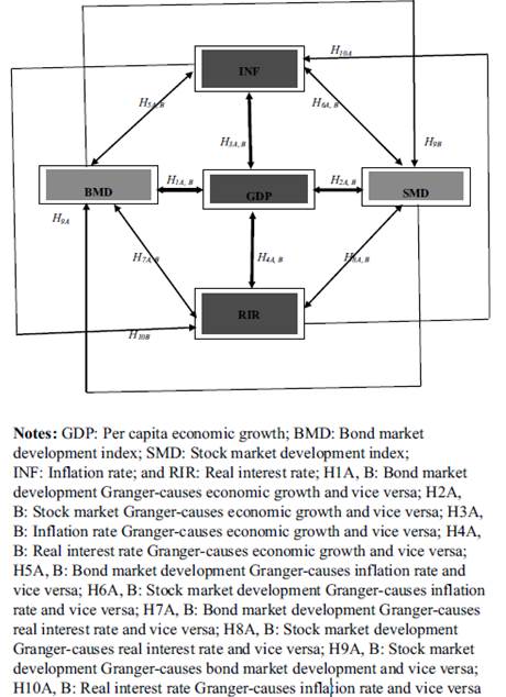
Figure 1 Possible causality between bond market development, stock market development, economic growth, inflation rate and real interest rate
We use the following vector error-correction model (VECM)[9] to examine the direction of Granger causal relationships between GDP, BMD, SMD, INF and RIR.
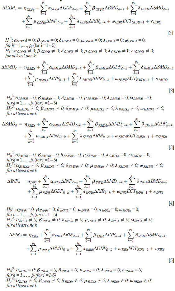
Where Δ is the first difference operator; i is the country, t is the year in the panel and « it is a normally distributed random error term for all i and t with a zero mean and a finite heterogeneous variance.
The ECTs are error-correction terms, derived from the cointegrating equations (see, for instance, Engle and Granger, 1987). The lagged ECTs represent the long-run dynamics, while the differenced variables represent the short-run dynamics between the variables. The above model is meaningful if the time series variables are I(1) and are cointegrated[10]. If the time series variables are I (1) and are not cointegrated, the lagged ECT component will bremoved in the estimation process. We look for both short-run and long-run causal relationships between GDP, BMD, SMD, INF and RIR. The short-run causal relationship is measured through F-statistics and the significance of the lagged changes in the independent variables, whereas the long-run causal relationship is measured through the significance of the t-test of the lagged ECTs. Based on equations (2)-(6), Table 4 presents the synopsis of various possible hypotheses concerning the causal relationships among the variables.
6. Empirical results and discussion
The empirical investigation starts with unit root and cointegration between five sets of variables: GDP, BMD, SMD, INF and RIR. Both the unit root test and cointegration tests are the pre-requisite for the Granger causality tests (see, for instance, Engle and Granger, 1987; Granger, 1988). The unit root test examines the order of integration [i.e. I (n), for n =1, 2,., N] where the time series variables attain stationarity, while cointegration tests examine the existence of long-run equilibrium relationships between the variables.
We use panel unit root tests to determine the degree, or order, of integration between GDP, BMD, SMD, INF and RIR. While several panel unit root tests are accessible to estimate, we use three different panel unit root tests: LLC, ADF and PP tests [the unit root tests proposed by Levin et al. (2002) and Maddala and Wu (1999)] to identify the order of integration of these variables. Because these panel unit root tests are widely used in many research papers and are described in advanced econometrics textbooks, we choose not to elaborate on them here.
Table 4 Hypotheses tested in this study
| Causal flows | Restrictions | |
|---|---|---|
| BMD => GDP | βGDPik≠ 0; ωGDPi ≠0 | |
| GDP => BMD | βMDik≠0; ωBMDi≠0 | |
| SMD => GDP | δDPik≠0; ωGDPi≠0 | |
| GDP => SMD | δSMDik≠0; ωSMDi≠0 | |
| INF => GDP | µGDPik≠0; ωGDPi≠0 | |
| GDP => INF | µINFik≠0; ωINFi≠0 | |
| RIR => GDP | λGDPik≠0; ωGDPi≠0 | |
| GDP => RIR | λRIRik≠0; ωRIRi≠0 | |
| SMD => BMD | δBMDik≠0; ωBMDi≠0 | |
| BMD => SMD | βSMDik≠0; ωSMDi≠0 | |
| INF => BMD | µBMDi≠0; ωBMDi≠0 | |
| BMD => INF | δINFik≠0; ωINFi≠0 | |
| RIR => BMD | λBMDik≠0; ωBMDi≠0 | |
| BMD => RIR | µRIRik≠0; ωRIRi≠0 | |
| INF => SMD | µSMDik≠0; ωSMDi≠0 | |
| SMD => INF | βINFik≠0; ωINFi≠0 | |
| RIR => SMD | λSMDik≠0; ωSMDi≠0 | |
| SMD => RIR | δRIRik≠0; ωRIRi≠0 | |
| RIR => INF | λINFik≠0; ωINFi≠0 | |
| INF => RIR | βRIRik≠0; ωRIRi≠0 | |
| Notes: GDP: Per capita economic growth; BMD: Bond market development index; SMD: Stock market development index; INF: Inflation rate; and RIR: Real interest rate | ||
| Source: Authors’ tabulations | ||
Table 5 shows the results of the panel unit root tests for each variable. These tests confirm that all the variables are (GDP, BMD, SMD, INF and RIR) integrated of order one, i.e. I (1). As the test-statistics of the unit root test at levels are below the critical values for all the various approaches, the null hypothesis of unit root at the 1 per cent significance level is accepted. However, as the test-statistics of the unit root test in first difference are above the critical values for all the approaches, the null hypothesis of unit root at the 1 per cent significance level is rejected so that the variables are integrated of order one (see the results in Table 5). These results reveal that there is the possibility of cointegration among per capita economic growth, bond market development, stock market development, inflation rate, and real interest rate.
Table 5 Results from panel unit root test
| Variable | GDP | BMD | SMD | INF | RIR |
|---|---|---|---|---|---|
| Sample 1: G-20 Developed countries | |||||
| Case 1: Level data | |||||
| LLC | -0.80 (0.21) | 3.35 (0.99) | 2.77 (0.99) | _0.61 (0.27) | _0.51 (0.17) |
| 10.3 (0.92 | 1.54 (1.00) | 2.28 (1.00) | 13.4 (0.77) | 22.7 (0.22) | |
| 17.8 (0.47) | 0.23 (1.00) | 1.89 (1.00) | 15.4 (0.64) | 31.79 (0.20) | |
| Case 2: First differenced data | |||||
| LLC | _11.7* (0.00) | _4.27* (0.00) | _7.34* (0.00) | _11.1* (0.00) | _8.35* (0.00) |
| ADF | 125.5* (0.00) | 69.23* (0.00) | 70.9* (0.00) | 116.2* (0.00) | 95.00* (0.00) |
| PP | 174.9* (0.00) | 69.57* (0.00) | 104.4* (0.00) | 164.9* (0.00) | 141.7* (0.00) |
| Sample 2: G-20 developing countries | |||||
| Case 1: Level data | |||||
| LLC | _0.122 (0.45) | 1.55 (0.94) | 1.57 (0.94) | -0.47 (0.30) | -0.11 (0.21) |
| ADF | 2.267 (0.97) | 3.73 (0.96) | 2.04 (0.99) | 13.76 (0.29) | 13.01 (0.20) |
| PP | 5.437 (0.86) | 1.27 (0.94) | 2.86 (0.98) | 10.97 (0.36) | 11.06 (0.23) |
| Case 2: First differenced data | |||||
| LLC | -31.1* (0.00) | -8.51* (0.00) | -5.90* (0.00) | -8.58* (0.00) | -12.92* (0.00) |
| ADF | 77.51* (0.00) | 50.59* (0.00) | 47.8* (0.00) | 71.75* (0.00) | 76.86* (0.00) |
| PP | 109.4* (0.00) | 59.2* (0.00) | 77.82* (0.00) | 100.06* (0.00) | 102.17* (0.00) |
| Sample 3: All G-20 countries | |||||
| Case 1: Level data | |||||
| LLC | -0.692 (0.24) | 3.676 (0.99) | 3.177 (0.99) | _1.015 (0.20) | _0.95 (0.26) |
| ADF | 13.6 (0.98) | 5.267 (1.00) | 4.323 (1.00) | 37.17 (0.15) | 35.71 (0.15) |
| PP | 23.23 (0.72) | 1.503 (1.00) | 4.744 (1.00) | 26.32 (0.55) | 42.85 (0.20) |
| Case 2: First differenced data | |||||
| LLC | _31.64* (0.00) | _8.96* (0.00) | _9.426* (0.00) | _13.67* (0.00) | _15.09* (0.00) |
| ADF | 202.9* (0.00) | 119.8* (0.00) | 118.7* (0.00) | 187.9* (0.00) | 171.9* (0.00) |
| PP | 284.3* (0.00) | 128.7* (0.00) | 182.2* (0.00) | 265.0* (0.00) | 243.87* (0.00) |
| Notes: GDP: Per capita economic growth; BMD: Bond market development index; SMD: Stock market development index; INF: Inflation rate; and RIR: Real interest rate; LLC: Levin-Lin-Chu statistics; ADF: Augmented Dickey-Fuller statistics; PP: Phillips-Perron statistics; the null hypothesis is that the variable follows a unit root process; *indicates significance at the 1% level; methods used are based on Levin et al. (2002); Maddala and Wu (1999) | |||||
| Source: Authors’ calculations | |||||
We use a panel cointegration test to determine the long-run equilibrium relationship between GDP, BMD, SMD, INF and RIR. While several panel cointegration tests are available, this paper uses the Pedroni panel cointegration test (Pedroni, 1999) to determine the existence of cointegration among these five series. The null hypothesis of no cointegration is based on seven different test statistics (Pedroni, 2000), which includes four individual panel statistics [panel v-statistic, panel r -statistic, panel t-statistic (non-parametric), and panel t- statistic (parametric)] and three group statistics [group r -statistic, group t-statistic (non- parametric), and group t-statistic (parametric)]. Because these test statistics are described in advanced econometrics textbooks, we choose not to describe them here.
Table 6 shows the results of the panel cointegration test. In nearly every case, the null hypothesis of no-cointegration is rejected by most of these test statistics at the 1 per cent level (see Table 6 for the cases: the G-20 developed countries, the G-20 developing countries, and the G-20 countries in total, respectively). Remarkably, this is true in all three samples. Hence, this confirms the existence of a long-run equilibrium relationship between the variables in the three cases that we study. We will comment on the exact nature of the long-run relationships below.
The findings presented above support the final step in our investigation, which is using a VECM approach to examine the nature of causal relationships among the five sets of variables. The existence of I (1) stationarity and cointegration among the variables implies the possibility of Granger causality among them. Hence, we conduct a Granger causality test, using a VECM and using equations (2)-(6). The results are shown in Table 7. We report the panel-Granger causality test results for both the short run, through the significance of the F-statistic, and the long run, through the significance of the lagged ECTs. The tests were conducted for 1, 5 and 10 per cent significance levels. The results for the long- and short-run Granger causality tests are described below.
Table 6 Results of Pedroni panel cointegration test
| Test statistics | No. intercept and no trend | Deterministic intercept only | Deterministic intercept and trend |
|---|---|---|---|
| Sample 1: G-20 developed countries | |||
| Panel v-Statistics | -0.81 (0.74) | _0.55 (0.74) | _1.50 (0.93) |
| Panel r - Statistics | -0.12 (0.25) | 1.04 (0.85) | 2.15 (0.98) |
| Panel PP- Statistics | -4.17* (0.00) | _5.03* (0.00) | _7.83* (0.00) |
| Panel ADF- Statistics | -234 (0.20 | _3.41 (0.00) | _2.14 (0.01) |
| Group r - Statistics | 1.78 (0.67) | 2.54 (0.99) | 3.47 (0.99) |
| Group PP- Statistics | _7.08* (0.00) | _7.57* (0.00) | _11.2* (0.00) |
| Group ADF- Statistics | _2.98* (0.00) | _3.07 (0.00) | _1.88*** (0.10) |
| Inference: Cointegrated | |||
| Sample 2: G-20 developing countries | |||
| Panel v-Statistics | _0.67 (0.75) | _0.64 (0.74) | _1.34 (0.91) |
| Panel r - Statistics | _0.67 (0.25 | 0.26 (0.60) | 0.69 (0.76) |
| Panel PP- Statistics | _3.88* (0.00) | _2.25* (0.00) | _3.30* (0.00) |
| Panel ADF- Statistics | _2.84* (0.00) | _3.32* (0.00) | _2.51* (0.01) |
| Group r - Statistics | 0.45 (0.67) | 1.37 (0.91) | 1.91 (0.97) |
| Group PP- Statistics | _5.81* (0.00) | _1.87** (0.03) | _2.23* (0.01) |
| Group ADF- Statistics | _2.22* (0.01) | _2.68* (0.00) | _0.91 (0.82) |
| Inference: Cointegrated | |||
| Sample 3: All G-20 countries | |||
| Panel v-Statistics | _1.07 (0.86) | _0.91 (0.82) | _2.10 (0.98) |
| Panel r - Statistics | _0.67 (0.25) | _0.83 (0.79) | 1.87 (0.97) |
| Panel PP- Statistics | _5.90* (0.00) | _4.44* (0.00) | _6.37* (0.00) |
| Panel ADF- Statistics | _2.11* (0.01) | _1.42*** (0.07) | _0.54 (0.29) |
| Group r - Statistics | 1.69 (0.96) | 2.85 (0.99) | 3.92 (0.99) |
| Group PP- Statistics | _9.15* (0.00) | _7.19* (0.00) | _10.3* (0.00) |
| Group ADF- Statistics | _3.17* (0.00) | _2.05** (0.05) | _2.28 (0.00) |
| Inference: Cointegrated | |||
| Notes: Variables and regions shown above are defined in the text. Natural log forms are used in our estimation; the null hypothesis is that the variables are not cointegrated; figures in square brackets are probability levels indicating significance; *indicates significance at the 1% level; **indicates significance at the 5% level; and ***indicates significance at the 10% level; ADF: Augmented Dickey-Fuller statistics; PP: Phillips-Perron statistics; the other statistics are defined in Pedroni (1999, 2000) | |||
| Source: Authors’ calculations | |||
6.1 Long-run causality
From Table 7, it is evident that when DGDP serves as the dependent variable, the lagged error-correction term (ECT-1) is statistically significant in all three samples at the conventional significance levels. This implies that GDP tends to converge to its long-run equilibrium path in response to changes in its regressors (BMD/SMD/INF/RIR). The significance of the ECT _1 coefficient in the DGDP equation in each of the three samples confirms the existence of a long-run equilibrium between real economic growth rate and its determinants, which are bond market development, stock market development, inflation rate, and the real rate of interest.
Table 7 Granger causality test resu
| Dependent variable | DGDP | DBMD | Independent variables DSMD | DINF | DRIR | Lagged ECT ECT -1 | |||
|---|---|---|---|---|---|---|---|---|---|
| Sample 1: G-20 developed countries | |||||||||
| DGDP | - | 31.45* (0.00) | 8.43* (0.00) | 22.19* (0.00) | 10.46* (0.00) | -0.15* (-5.79) | |||
| DBMD | 3.831** (0.05) | - | 6.03* (0.00) | 4.74** (0.05) | 3.69* (0.00) | -0.02* (-4.271) | |||
| DSMD | 3.568** (0.05) | 8.41* (0.00) | - | 0.49 (0.00) | 3.535** (0.00) | -0.04* (-4.189) | |||
| DINF | 6.451** (0.00) | 1.255 (0.74) | 3.912** (0.00) | - | 0.989 (0.80) | - 0.05* (-3.83) | |||
| DRIR | 6.31** (0.00) | 7.677* (0.00) | 7.444* (0.00) | 8.35* (0.00) | - | -0.002 (-0.23) | |||
| Sample 2: G-20 developing countries | |||||||||
| DGDP | - | 8.123* (0.00) | 5.967* (0.00) | 3.872** (0.05) | 4.866* (0.00) | -0.052* (-6.22) | |||
| DBMD | 4.822** (0.05) | (0.00) | 9.804* (0.00) | 8.640* (0.90) | 8.171* (0.00) | -0.016 (-1.783) | |||
| DSMD | 3.799** (0.02) | 2.169 (0.52) | - | 1.251 (0.89) | 1.874 (0.56) | -0.014 (-0.69) | |||
| DINF | 16.56* (0.00) | 10.53* (0.00) | 36.7* (0.00) | - | 9.634* (0.00) | -0.347* (-4.32) | |||
| DRIR | 6.032* (0.10) | 3.251** (0.10) | 7.88* (0.00) | 2.131 (0.78) | - | -0.003 (-0.012) | |||
| Sample 3: All G-20 countries | |||||||||
| DGDP - | 30.11* (0.00) | 14.85* (0.00) | 11.65* (0.00) | 11.23* (0.00) | -0.50* (-4.356) | ||||
| DBMD | 12.9* (0.00) | - | 14.22* (0.00) | 2.272 (0.00) | 7.68* (0.00) | -0.03 (-1.19) | |||
| DSMD | 11.91* (0.00) 1.72 (0.00) - | 1.72 (0.00) | - | 2.153 (0.00) | 7.049* (0.00) | -0.15* (-3.12) | |||
| DINF | 4.65** (0.00) 15.71* (0.00) 38.8* (0.00) | 15.71* (0.00) | 38.8* (0.00) | - | 6.889* (0.00) | -0.07* (-4.2) | |||
| DRIR | 5.24** (0.00) 11.8* (0.00) 13.62* (0.00) | 11.8* (0.00) | 13.62* (0.00) | 12.61* (0.00) | - | -0.01 (-0.15) | |||
| Notes: GDP: Per capita economic growth; BMD: Bond market development index; SMD: Stock market development index; INF: Inflation rate; RIR: Real interest rate; and ECT_1: lagged error-correction term; The study uses the Akaike information criterion (AIC) and Schwarz information criterion (SIC) to determine the optimum lag length. Like the standard information criteria, a smaller AIC (or SIC) indicates a better fit of the model to the data; values in square brackets indicate probabilities for F statistics, while those in parentheses are t statistics; *and **indicate that the parameter estimates are significant at the 1% and 5% levels, respectively | |||||||||
| Source: Authors’ calculations | |||||||||
The estimated lagged ECTs, Samples 1-3, all carry negative signs, as expected. Thisimplies that the change in the level of economic growth (DGDP) rapidly responds to any deviation in the long-run or short-run disequilibrium, for the t-1 period. In other words, the effect of an instantaneous shock to bond market development, stock market development, inflation rate and the real interest rate on economic growth will be completely adjusted in the long-run. However, the return to equilibrium occurs at different rates: 22 per cent in Sample 1, 13 per cent in Sample 2 and 50 per cent in Sample 3. The empirical results allow us to infer that if there is any deviation from the long-run equilibrium relationship between the chosen economic variables, real economic growth is found to respond to correct this deviation.
From Table 7, when DINF serves as the dependent variable, the lagged error-correction term (ECT_1) is also statistically significant in all three samples at the conventional significance levels. This implies that INF tends to converge to its long-run equilibrium path in response to changes in its regressors (GDP/BMD/SMD/RIR). The significance of the ECT- 1 coefficient in the DINF equation in each of the three samples confirms the existence of a long-run equilibrium between inflation rate and their determinants, which are bond market development, stock market development, real economic growth rate and real rate of interest. In this case, the return to equilibrium occurs at different rates: 15 per cent in Sample 1, 88 per cent in Sample 2 and 66 per cent in Sample 3.
The empirical results equally allow us to infer that if there is any deviation from the longrun equilibrium relationship between the chosen economic variables, then the rate of inflation is found to respond to correct this deviation. Similarly, when DBMD/DSMD serves as the dependent variables, the lagged error correction term (ECT_1) is statistically significant but only in the sample of the G-20 developed countries. In this case, we can infer that both BMD and SMD tend to converge to their long-run equilibrium path in response to changes in their regressors (GDP/INF/RIR). The significance of the ECT _1 coefficient in the DBMD/DSMD equation in Sample 1 confirms the existence of a long-run equilibrium between bond market development (or stock market development) and its determinants, which are the other variables. In this case, the return to equilibrium occurs at different rates: 2 per cent and 3 per cent, respectively.
The lagged error-correction terms in the DRIR equations in Table 7 are not statistically significant in any of the three samples. Hence, the real interest rate shows no evidence of correcting any deviations to the long-run equilibrium.
6.2 Short-run causality
In contrast to the fairly uniform long-run Granger causality results, our study reveals a divergent set of short-run causality results between the five variables. These results are summarized in Table 8 and are presented below.
Table 8 The summary of short-run granger causality between bond market development, stock market development, economic growth, inflation rate, and real interest rate in the G-20 countries
| Causal relationships tested in the model | Direction of relationships observed in the G-20 developed countries | Direction of relationships observed in the G-20 developing countries | Direction of relationships observed in the G-20 countries as a whole |
|---|---|---|---|
| BMD vs GDP | BMD <=> GDP | BMD <=> GDP | BMD <=> GDP |
| SMD vs GDP | SMD <=> GDP | SMD <=> GDP | SMD <=> GDP |
| INF vs GDP | INF <=> GDP | INF <= >GDP | INF <=> GDP |
| RIR vs GDP | RIR <=> GDP | RIR <=> GDP | RIR <=> GDP |
| SMD vs BMD | SMD <=> BMD | SMD => BMD | SMD => BMD |
| INF vs BMD | INF => BMD | INF <=> BMD | INF <= BMD |
| RIR vs BMD | RIR <=> BMD | RIR <=> BMD | RIR <=> BMD |
| INF vs SMD | INF <= SMD | INF <= SMD | INF <= SMD |
| RIR vs SMD | RIR <=> SMD | RIR <= SMD | RIR <=> SMD |
| RIR vs INF | RIR <= INF | RIR => INF | RIR <=> INF |
| Notes: GDP: Per capita economic growth; BMD: Bond market development index; SMD: Stock market development index; INF: Inflation rate; and RIR: Real interest rate; =>/<=: unidirectional causality; and <=>: Bidirectional causality | |||
| Source: Authors’ tabulations | |||
6.2.1 Sample 1: G-20 developed countries.
It shows the existence of bidirectional causality between bond market development and economic growth [BMD <=> GDP], stock market development and economic growth [SMD <=> GDP], inflation rate and economic growth [INF <=> GDP], real interest rate and economic growth [RIR <=> GDP], bond market development and stock market development [BMD <=> SMD], bond market development and real interest rate [BMD <=> RIR] and stock market development and real interest rate [SMD <=> RIR]. Additionally, we find unidirectional causality from the inflation rate to the bond market development [INF => BMD], from stock market development to inflation rate [INF <= SMD], and from the inflation rate to the real interest rate [INF => RIR].
6.2.2 Sample 2: G-20 developing countries.
It shows the existence of bidirectional causality between the bond market development and the economic growth [BMD <=> GDP], stock market development and economic growth [SMD <=> GDP], inflation rate and economic growth [INF <=> GDP], real interest rate and economic growth [RIR <=> GDP], and bond market development and real interest rate [BMD <=> RIR]. Additionally, we find unidirectional causality from stock market development to bond market development [BMD <= SMD], from stock market development to real interest rate [SMD => RIR], from bond market development to inflation rate [INF <= BMD], from stock market development to inflation rate [INF <= SMD] and from real interest rate to inflation rate [INF <= RIR].
6.2.3 Sample 3: all G-20 countries.
It shows the existence of bidirectional causality between bond market development and economic growth [BMD <=> GDP], stock market development and economic growth [SMD <=> GDP], inflation rate and economic growth [INF <=> GDP], real interest rate and economic growth [RIR <=> GDP], bond market development and real interest rate [BMD <=> RIR], stock market development and real interest rate [SMD <=> RIR] and real interest rate and inflation rate [INF <=> RIR]. Moreover, we find unidirectional causality from stock market development to bond market development [BMD <= SMD], from bond market development to inflation rate [INF <= BMD], and from stock market development to inflation rate [INF <= SMD].
6.3 Innovation accounting
Finally, we use innovation accounting to assess the nature of responses to perturbations of the different variables in the system of equations. Towards this end, we use generalized impulse response functions (GIRFs). The use of GIRFs is to trace the effect of a one-off shock to one of the innovations on the current and future values of the endogenous variables. The key consequence of the GIRFs is that the responses are invariant to any re-ordering of the variables in the VECM and, as orthogonality is not imposed, it allows for meaningful interpretation of the initial impact response of each variable to shocks in any other variables.
Figures 2, 3 and 4 show the GIRFs of the three panel VAR[11] models pertaining to our Samples 1-3. Our discussion of the impulse response functions centers on the responses of economic growth, bond market development, stock market development, inflation rate and real interest rate to their own and other shocks. In particular, the GIRFs indicate how long and to what extent bond market development, stock market development, and the other two macroeconomic determinants react to changes in the economic growth in the panel of the G-20 countries.
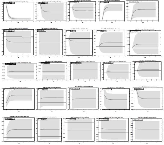
Notes: GDP: Per capita economic growth rate; BMD: Composite index of bond market development; SMD: Composite index of stock market development; INF: Inflation rate; RIR: Real interest rate.
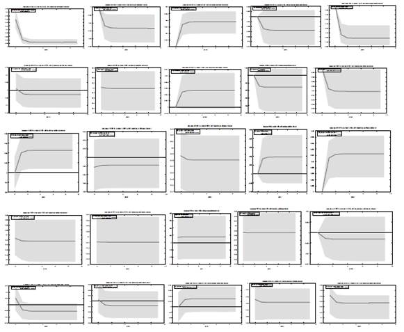
Figure 3 Plot of generalized impulse response functions for the G-20 developing countries (Sample 2)
Notes: GDP: Per capita economic growth rate; BMD: Composite index of bond market development; SMD: Composite index of stock market development; INF: Inflation rate; RIR: Real interest rate
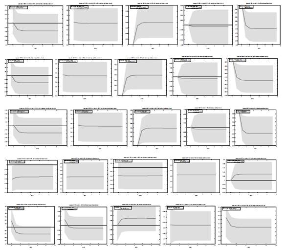
The significance of the impulse response is largely determined using confidence bands. Figures 2-4 display the GIRFs of the five vector error correction models. The shaded area in these figures represents the confidence bands. When the horizontal curves in the GIRFs fall between the confidence bands, the impulse responses are statistically significant. In other words, the null hypothesis of “no effects of a particular shock” on the specific variable cannot be rejected. Our discussion of the impulse response functions mainly centers on the responses of economic growth, bond market development, stock market development, inflation rate and real interest rate to their own and other shocks. For comparative analysis, we report the GIRFs to one-standard-error confidence bands (roughly equal to 95 per cent confidence bands) and the responses are very similar to those which we obtained using Cholesky one standard innovation.
In sum, Figure 2 shows the responses of all the variables to a one standard deviation shock in other variables. In each case, the stock market activity variable is found to display an initial cyclical response to an exogenous shock, albeit in varying degrees. However, the responses of all of the variables to exogenous shocks stabilize in around five years. In Figures 3 and 4, the responses of all variables to an exogenous shock are found to be highly similar, thereby signifying that for the three different measures of stock market depth, theesponses of variables are no different.
Some other features of these results, though not reported, deserve mention. First, we performed diagnostic checks in our three panel VAR models using our three samples. These included the autocorrelation Lagrange multiplier (LM) test, the normality test, and the White heteroskedasticity test. Second, we conducted a sensitivity analysis by using individual bond market indicators (PUB, PRB and INB)
7. Conclusion and policy implications
In this paper, we have examined the Granger causal relationships between bond market development, stock market development and economic growth in the presence of two additional macroeconomic covariates: inflation rate and real interest rate. Using panel data of the G-20 countries from 1991 to 2016, we found that both bond market development and stock market development are cointegrated with economic growth, inflation rate, and real interest rate. The panel Granger causality test further confirms that, among other things, bond market development, stock market development, economic growth, inflation rate, and real interest rate Granger cause economic growth in the long run. However, our short-run Granger causality results revealed a wide range of short-run adjustment dynamics between these five variables, including the possibility of feedback between them in several instances.
These results demonstrate that studies on economic growth that do not consider bond market development, stock market development, inflation rate, and real interest rate will offer potentially biased results. The partial findings would not only suffer the downside consequences of a missing-variable bias but would also distort and mislead policymakers. If policymakers intend to stimulate economic growth, then they should consider the codevelopment of financial markets, meaning fostering simultaneous development in both the bond market and the stock market. Clearly, the bond market and stock market development are drivers of economic growth; both developments complement each other and positively impact on macroeconomic stability.
In sum, by establishing the linkages between bond market development, stock market development, economic growth and other macroeconomic covariates, we show that the G-20 countries wishing to sustain economic growth, in the long run, should focus attention on developing their financial markets as well as maintaining macroeconomic stability in terms of interest rate and inflation rate. Moreover, the governments of these countries should strive to develop their economies, which will, in turn, lead to an improved bond market, stock market and further macroeconomic stability. These measures will have a virtuous influence on the overall development of financial markets and overall economic development of the country in general.
Notes
1. Financial development means the factors, policies and institutions that lead to effective financial intermediation and markets, as well as deep and broad access to capital and financial services(IMF, 2005).
2. Although different economists assign different degrees of importance to financial development, its contribution in economic growth can be theoretically postulated and has been supported by considerable empirical evidence (Law and Singh, 2014; Menyah et al., 2014; Ngare et al., 2014; Herwartz and Walle, 2014; Samargandi et al., 2014; Pradhan et al., 2013a).
3. Bond market development represents the intensity of public, private and international bond markets. The research on this area remains limited in comparison with banks and stock markets (see, for instance, Mu et al., 2013; Sharma, 2001).
4. A Granger causality test reports on both short- and long-run effects and hence is of special interest to policymakers (Marques et al., 2013).
5. Financial development includes both bond and stock market developments in our paper but is taken differently in most papers to include development in the stock market, the bond market or even the banking sector.
6. In the standard finance literature, both bond markets and stock markets developments areusually well interconnected with near-concomitant changes in the interest rate and inflation rate (Lee and Hsieh, 2014; Rahman and Mustafa, 1997).
7. The G-20 consists of 19 member countries plus the European Union (EU), which is represented by the President of the European Council and by the European Central Bank. Thus, although we look at the G-20, within this group of important industrialized and developing economies, we observe only 19 member nations, which are used for our analysis. The inclusion of the EU, the twentieth member, would have meant double-counting France, Germany, Italy and the UK.
8. The data were obtained from the World Development Indicators and Financial Development and Structure Dataset, both published by the World Bank. The period of our study is chosen based on data availability.
9. The estimation of VECM follows the structure of Holtz-Eakin et al. (1988) and Arellano and Bond (1991).
10. The estimation of VECM follows the procedures set out in Holtz-Eakin et al. (1988) and Arellano and Bond (1991).
11. VAR denotes vector autoregressive.

