


 English (pdf)
 Article in xml format
 Article references
 Send this article by e-mail
 Cited by SciELO
  Similars in
SciELO
Similars in
SciELO 
 Permalink
1. Introduction
According to Barbier, E. B. (2003) most of the Economists recognize that by including physical capital natural and environmental resources should also be observed because these are also the most important economic assets. There are three debates covered from different dimensions have arisen recently related to the role of natural resources in economic growth or economic development. Firstly, does the environment plays a vital role in sustainable development and human welfare? If the concept is true, then is there any specific “compensation rules” essential to ensure that the future welfare of the society is not deteriorated by natural resources reduction today? Secondly, the environmental Kuznets curve theory has promoted the empirical finding of an “inverted U” shaped relationship between environmental pollution indicators. Does the existence of such type of relationship of EKC advocate that environmental degradation will ultimately reduce with growth? Finally, modern economic theories questioned based on empirical findings whether low-income economies which are endowed with natural resources develop quickly as compared to the economies that are poor in sense of natural resources? The most important question filtered from all dimensions of the debate is how natural resources play a role in the economic growth of the economy?
Water is a huge natural resource and it can be regarded as the essential ingredient and the source of life on earth. Life is tied to water as it is attached to air and food. Until the past few decades, the resources of freshwater were considered to be more than satisfactory for human needs, however, with the growing rate of population, freshwater has become scarce at an accelerated rate. Access to water has always been considered essential to socio-economic development, sound environment, the strength of societies and civilizations and the survival of human race itself. In less-developed nations, a huge number of individuals, most of them ladies, walk miles every day to discover the water they need and convey it back home. However, water availability has not got the consideration it deserves in a worldwide discussion of the feasible utilization of natural resources. It has been analysed even less with regards to population growth.
Water resources are a vital element for production around the world. Many nations face water accessibility issues in addition to dry spells and ground-water depletion. Besides, water in dry zones is scarce to the point that it is no more conceivable to take care of the demand without surpassing economical amount and quality use rates. As demands from all divisions are required to keep growing, the conflicts over water utilization will worsen soon. The world, in general, is currently facing the threat of water shortage. The growing demand driven by population growth and economic development creates strong competition for water between different areas. Nowadays, media raises their voice to aware people about water shortage that we can face in the coming decades. It is predicted that 66% of the total population would be living in water-stressed areas by 2025. Water is renewable only if well managed. Water resources should be managed efficiently and on equitable basis otherwise, it can raise a serious challenge to achieve sustainable growth.
2. Literature review
Water is fundamental for human life, food, environment, and economic growth. Absence of access to water adversely influences socio-economic stability. Environmental change due to the greenhouse impact has flourished as one of the most important environmental problems for the 21st century. Emissions resulting out of the human activities are increasing the atmospheric concentrations of dangerous gases resulting in an extra warning on the earth surface. Water scarcity is achieving alarming dimensions considering the extremely rapid population growth. Water would not be effectively accessible to support the new generation and socioeconomic development. The shortage of water results in a significant reduction in the growth of the economy. Economic activities include production and consumption processes that cannot remain unravelled beyond their environment. Therefore, the impacts on the surroundings increase with economic development. However, the contradiction into the procedure of economic growth versus its fixed consequences on non-renewable resources makes the relationship a sophisticated one.
Panayotou (1997) examined the Environmental Kuznets Curve by utilizing the principle factors, like sulfur dioxide, population density, policy variable, annual growth rate, and GDP. The example included 30 developed and developing nations for the period 1982-94. On account of the surrounding SO2 levels, he found that the nature of the policies and organizations could altogether decrease ecological corruption at low pay levels and accelerate change at higher wage levels. He found developing proof that ecological corruption limits conceivable development outcomes. He predicted that out of 8 billion individuals, 5 billion individuals will endure the water worry in 2025. He proposed that better arrangements, for instance, secure property rights, a better requirement of agreements and successful ecological directions, could straighten the natural Kuznets bend and lessen the natural cost of monetary development.
Akram (2012) studied the impact on the environment due to the economic development in the selected Asian countries for the years 1972-2009. The results showed that the growth of the economy was contrarily influenced by the means of changes in temperature, perception, and the growth of population, while urbanization and human advancement invigorated the growth of the economy. Agriculture was the almost powerless part to contribute to the environmental change, while, assembling was the slightest influenced division. The findings also showed that the economic growth was contrarily influenced by the means of change in the temperature, precipitation and growth of population, while urbanization and human improvement empowered the economic growth.
Choumert et al. (2013) studied the variance of EKC and the relationship between economic growth and deforestation. The work used parameters, like, econometric methodology, the measure of deforestation, geographical region, and presence of control factors for investigating EKC. A defining moment was identified after 2001 and it was established that EKC would not blur until a hypothetical option was given.
The study analysed the association between them for eleven countries over the period 1981-2009, using panel unit roots, co-integration in heterogeneous panels and panel causality test. They checked up that there was some positive long-run relationship among the emissions of CO2, electric power and energy use in GDP. There was a bi-directional causality between the emissions of carbon dioxide and the utilization of electric power. This study also analysed the greenhouse gases emissions and employed ordinary least squares and dynamic ordinary least squares to evaluate the relevant coefficients.
The hypothesis of structural change and Environmental Kuznets Curve was analysed by Marsiglio et al. (2016). The study constructed a standard Balanced Growth Path (BGP) for the flow of wages, structural changes, and pollution. A modified U-shaped income-pollution association occurred as a reaction to the structural changes. It was shown that the negative relationship between income and pollution was a temporary occurrence, while in the long run, pollution would increment with the expansion in income.
3. Methodology
3.1 Data collection
In this study, just the case of Pakistan was considered to find out the relationship between water, economic growth, and the environmental change.
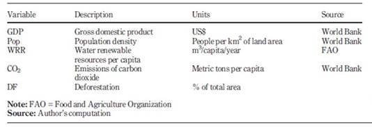
Total five variables are used in this study that is GDP, population density, water renewable resources, deforestation and the emissions of CO2, based on time-series data from 1972-2016. The annual data is collected from World Development Indicators, Food and Agriculture Organization, and Pakistan Economic Survey. To make results linear and all variables of the magnitude order, transformation of all variables to logarithm has been done.
Sample size plays an imperative part in getting solid outcomes; the point behind the determination of ideal example size is to guarantee a satisfactory force of measurable hugeness of discoveries in relationship (Nucu, 2011). For getting critical outcomes, as a general guideline, 80% example size is required (Agalega and Antwi, 2013).
This study uses the time series data from 1972 to 2016 and the information set covers 45 observations. If the sample size is large, then there is less chance of the spurious results. This period is picked because of its remarkableness to Pakistan’s Economic Recovery Program. It is moreover picked as an aftereffect of the accessibility of data of the choice variables. Henceforth, the present study satisfies the states of ideal example estimate, having more than 80% perception. In this way, the sample size is satisfactory and colossal to achieve the targets in the study.
Descriptive statistics give the basic summaries of the data of the variables under consideration. These statistics are used to describe the characteristics of data. See Table 1 for the results of descriptive statistic on a logarithmic scale.
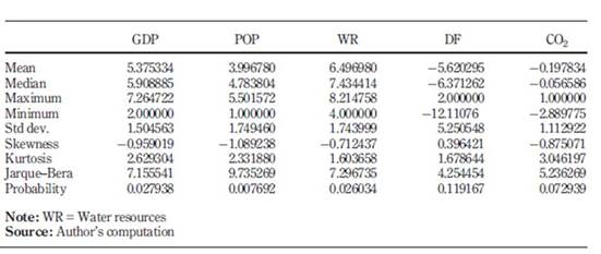
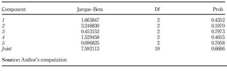
The table represents the detailed investigation of the variables which includes 45 observations from 1972 to 2016. It can be seen that the mean value of GDP is 5.38 with a standard deviation of 1.50 and maximum and minimum values of 7.26 and 2, respectively. Residuals for GDP variable are left-skewed, and on the base of kurtosis, it can be seen that the GDP is leptokurtic having a long tail. The calculated statistics of Jarque-Bera and corresponding p-values are used for testing the normality assumption. It demonstrates that the residuals of the GDP variable are normally distributed. The null hypothesis of normality test is that residuals are normally distributed, while the probability value is more than 5%. Subsequently, we acknowledge the alternative hypothesis that residuals are not normally distributed, and still, we can accept the model.
The mean value of the population density is 4 with a standard deviation of 1.7 with maximum and minimum values of 5.50 and 1, respectively. The average value of water renewable resources is 6.5, with a standard deviation of 1.74. Further, deforestation and emissions of CO2 have average values of -5.62 and -0.2, with standard deviation of 5.25 and 1.11, respectively. Water renewable resources and emission of CO2 are negatively skewed and not normally distributed, while the variable deforestation is positively skewed and has a normal distribution. Additionally, on the base of kurtosis, it can be seen that all variables are leptokurtic having a long tail (see Table 2).
As the >data on deforestation rate in Pakistan is not publicly available, it is calculated through the formula given by Puyravaud (2003):
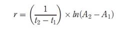
3.2 The model
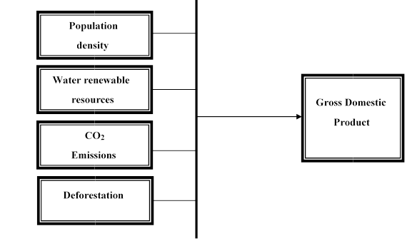
Gross Domestic Product (GDP), Population density (Pop), Water Renewable Resources (WRR) per capita, emissions of CO2 and Deforestation (DF) are being utilized as variables in the present study. This study is based on time series data, for the period time of 1972-2016. This research proposed GDP as a dependent variable, while population density, water renewable resources per capita, emissions of CO2 and deforestation taken as independent variables. The functional form of the model is the following:
𝑮𝑫𝑷 = (𝐏𝐨𝐩, 𝐖𝐑𝐑, 𝐂𝐎𝟐 𝐞𝐦𝐢𝐬𝐬𝐢𝐨𝐧𝐬, 𝐃𝐅) (2)
See Figure 1 for the research model.
3.3 Unit Root Tests
Time series data should be constant/stationary over time otherwise results would be misleading A stationary series is characterized as a series that tends to come back to its mean value and fluctuate round it within a consistent range, while a non-stationary series is characterized as a series whose techniques vary at various focuses in time and variance increases with the sample size. Stationarity checking is essential for the development of the econometric study. It is imperative to check for stationarity before moving towards model estimation. There are many tests to watch that problem, but the most standard test is augmented Dickey and Fuller (1979) test that includes extra lags for the dependent variable to expel serial autocorrelation, which can be decided on the base of AIC and SBC criteria.
Δ𝒚𝒕=α+ 𝜷𝒕 + γ𝒚𝒕−𝟏 +δ𝚫𝐲𝒕−𝟏+……. +δ𝒑𝒕−𝟏𝚫𝐲𝒕−𝒑+𝟏 + έ𝒕 (3)
Where α is a constant, β the coefficient, t is time trend and p the lag order of the auto regressive process.
3.4 Johansen Fisher Panel Cointegration Test
After testing the stationarity of the variables, if all modelled variables integrated on the same order then cointegration should be tested. It is the mandatory step before going towards the econometric technique. Cointegration predicts the existence or inexistence of long-run association between variables.
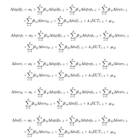
3.5 Vector Error Correction Model
To recognize the direction of the short run as well as long-run causality, we consider VECM. VECM is the extensive form of Error Correction Term. VECM use when there are two or more than two variables in the model which are stationary on the 1st difference. The VECM or vector error correction model looks like a VAR model, no doubt VECM is a VAR model is unrestricted VAR whereas VECM is restricted VAR. In the past, researchers, economists and other specialists used VECM TO apply simple regression, but in this case, it is said that the utilization of VECM without data stationarity is not suitable.
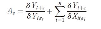
3.6 Impulse response
Innovation, which measures the impact of a one-unit increment in the white noise vector of the GDP or other variables referred to as impulse response function (Sims, 1980 and Verbeek, 2008).
3.7 Variance decomposition
In short, variance decomposition refers to the contribution of each innovation of the forecast error associated with the forecast of each variable. It was introduced by Sims (1980) to understand the VAR model. It isolates the variance of forecast error for each variable into parts.
4. Empirical analysis
4.1 Unit Root Test
Table 3
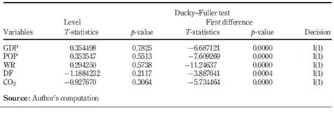
Null hypothesis: there is no unit root.
Table 3 represents the results of the test of unit root for all variables. If the absolute value of the Augmented Dicky Fuller (ADF) test is smaller than a certain value like 1% or 5% level of significance, we cannot reject the null hypothesis. According to ADF unit root results, the order of integration of all variables is I (1) with constant. It means all the dependent variables are integrated at first difference and none of the variables are integrated at the second difference. Hence, the null hypothesis is rejected because there is no trend in data. So, the appropriate technique for co-integration is the Johansen Co-Integration technique.
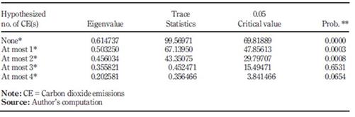
4.2 Johansen Fisher Cointegration Test
Table 4 demonstrates the null hypothesis of no co-integrating vector for 1-4 co-integrated vectors, under the trace and eigenvalue test. The null hypothesis in the case of none means there is no co-integration equations, at most one carries almost one co-integration equation, at most 2,3 and 4 suggests there is almost 2,3 and 4 co-integration equation respectively. The results recommended three co-integration equations and there is a clear rejection of the null hypothesis and conclude that the variables can move together over the long run. Hence, it is discovered that the VECM model should be preferred. See Table 4 for Johansen Fisher cointegration results.
All the variables under consideration in this study are stationary at first difference as well as they have the long-term co-integration. VECM is a fitted model to investigate whether there exists a long run as well as a short run relationship among the variables or not.
The two long run co-integration are as follows:
GDP = 8.998712 + 0.3344*ln(POP) + 0.450647*ln(WR) + 0.127821*DF + 0.802420*CO2 (4)
GDP = 8.998712 - 0.3344*ln(POP) - 0.450647*ln(WR) - 0.127821*DF -0.802420*CO2 (5)
Look at Table 5 to find the long run results of VCEM.
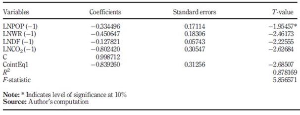
While interpreting VECM results, we have to reverse the signs of our coefficients in order to make the equation equal to zero. So, in the first equation, the coefficient sign is as it is, while in the latter one, signs are reversed.
Table 5 for VECM reports long-run coefficients, standard errors, and t-values. The coefficient of ECT(α) can be interpreted as the rate of shock convergence in the current period towards the equilibrium in the next period. This value must lie between 0 and -1, as 0 shows no adjustment, while -1 represents 100% adjustment. Our results show a value of -0.84, which means 84% speed of adjustment of the dependent variable can move towards equilibrium in one year from now.
The findings of the study demonstrate that all variables have a negative and significant relationship over the long run at 5% level of significance. It is observed that 1% in population accordingly will degrade GDP by 0.334496%. Correspondingly, a 1% increase of water renewable resources will degrade GDP by 0.450647%. Findings are aligning with the study of. Afzal (2009), Jiang (2009) and Whertel and Liu (2016). Moreover, a 1% increase in deforestation will diminish GDP by 0.127821%. The findings are aligning with the study of Koop and Tole (2001) and Kahuthu (2006). If we increase 1% CO2, GDP will be reduced by 0.802420%, confirming the findings in York (2012) and Kahuthu (2006.
Table 5 shows the R-squared value of 0.87 demonstrating that 87% variation in the dependent variable due to projected explanatory variables, while a 19% variation due to the missing factors in the model. F-statistics with 5.86 value shows that the overall model is good. The results show the effects of long-run yet, they also permit to investigate the short-run impact.
Short-run Granger Causality Test
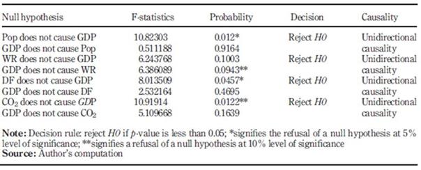
After the VECM model, the Granger causality test is utilized to determine the direction of the variables and the GDP of Pakistan. Table 6 summarizes the results.
Table 6 shows that there is a unidirectional causality running between all variables in the short run, predicting that all variables are Granger cause to GDP.
4.4 Impulse Response Function
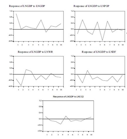
Impulses responses are graphically represented in Figure 2. Look at Table 7 to get an evaluation of impulse response function. Also, have a look at Figure 2 for a graphical representation of impulse response function.
GDP gives a negative response because of 1 standard deviation shock to the population in the first period. In the second period, it becomes positive and negative again in 3rd, 4th, 6th, 8th and 10th period. It remains positive in 5th, 7th and 9th period due to a shock to population. 1 standard deviation shock to the water resources demonstrates that GDP responds positively to water resources for the periods 1, 2, 5, 6, 7, 10 except the periods 2, 3 and 8. When the impulse is deforestation, then the response of the first two periods of GDP is negative. For the 3rd period, it becomes positive, but after that, with each impulse, GDP responds negatively to deforestation.
When the impulse is emissions of CO2, then, in the first period, the response of GDP is positive, but then for the next three periods, it becomes negative, and again positive for the next period and stays negative till period.
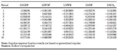
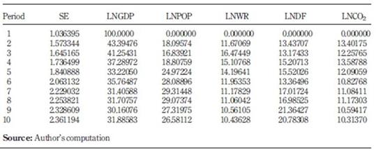
4.5 Forecast error variance decomposition
Table 8 presents that in the primary time period; the Gross Domestic Product characteristics 100% of its change due to its own shock rather than any other variable. But, in the second period, forecast error for GDP attributes 11.67% owing to water renewable resources and 18.10% due to population. Period 3 demonstrates that the variation in GDP is not only due to water renewable resources (16.47%), but also due to population, deforestation and CO2 emissions, by factors of 13.17%, 13.44% and 13.40%, respectively. In period 4, variation in GDP is 37.29% due to GDP own shock, while water renewable recourses, population, deforestation, and CO2 emissions cause 15.10%, 18.81%, 15.21%, and 13.59% variation, respectively. Maximum fluctuation in GDP is observed in period 5 due to its own shock (33.22%), while 24.97%, 14.20%, 15.52%, and 12.09% variation is observed due to water renewable recourses, population, deforestation, and CO2 emissions, respectively. Further, it can be clearly seen that the difference in GDP due to its own shock declines because of the population increase during the time period under study.
4.6 Model Stability Test. Inverse root of autoregressive characteristic polynomial of the estimated VAR model:
If the evaluated VAR and VECM are stable, then all the coefficients must be less than 1, i.e., means inside the unit circle, otherwise certain results are not valid. Look at Figure 3 to check the model stability diagnostic.
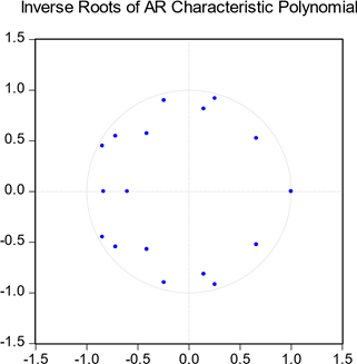
In Figure 3, all the dots inside the circle are regarded as stable.
4.7 Diagnostic tests
To examine the robustness of the selected model, this work utilizes necessary diagnostic tests, which are following:
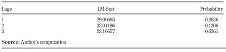
4.7.1 Autocorrelation
To keep away from serial correlation, we have chosen lag 3 as ideal. Please see Table 9 to check the serial correlation diagnostic results.
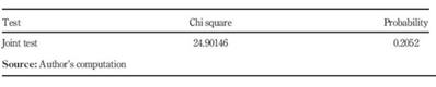
4.7.2 Heteroscedasticity Test
Table 10 presents the outcomes of the heteroscedasticity with the null hypothesis of homoscedasticity. If the probability value of heteroscedasticity test comes more than 5%, then it is the confirmation of non-appearance of heteroscedasticity issue in the model. As the results show more than heteroscedasticity 5%, so we can acknowledge the null hypothesis of homoscedasticity.
4.7.3 Normality test
Please have a look at Table 11 for normality test results.
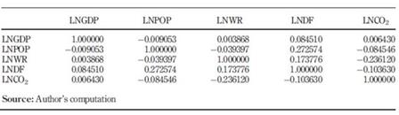
4.7.4 Multicollinearity Test
Table 12 shows the aftereffects of the Pearson correlation test. It can be performed for various purposes. We can utilize it to know the quality of the relationship among variables or to check the multicollinearity among the variables. If coefficients values are more than 0.8, it demonstrates the multicollinearity issue. Our results show that all coefficient values are less than 0.8, which is the proof that the model is free from multicollinearity. Please see Table 12 for multicollinearity test.
4.8 Lag Exclusion Wald Test
This test is carried out for each lag in VAR. The Wald statistics for the joint significance of all variables are reported for every equation independently and together for each lag in Table 13.
The numbers written in [ ] are p-values. Please see Table 13 for Lags exclusion Wald test.
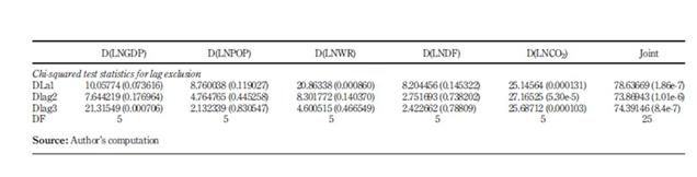
The results demonstrate that with 3 lags, we are getting a significant impact on the variables.
Thus, this test affirms that we must utilize 3 lags as an ideal lag length.
5. Conclusion and discussion
5.1 Environmental Kuznets Curve in Pakistan
Figure 4 represents the Environmental Kuznets curve for CO2 emissions in Pakistan for the period 1972-2016. The graph is generated using the software Stata.
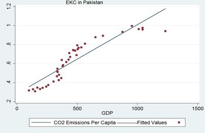
The graph shows no evidence of exact inverse U shape. It indicates that the current year’s pollution tends to decrease with higher economic growth. It seems like the Environmental Kuznets Curve does not hold in the case for Pakistan. The pollution level increases as the economy grows. There exists no turning point through which we can say the existence of EKC. However, in the recent current years, the pollution level tends to decrease and may lead to the U shaped curve in the future. The reason may be that the industrial sector, the most polluting sector, contribute a small amount towards the GDP of Pakistan. In Pakistan, the major source of CO2 emissions are industries and the share of industrial products in GDP of Pakistan is just around 20.30% according to Pakistan Economic Survey 2014. Although, the contribution of the service sector is much higher (58.8%), yet this sector is causing relatively less pollution. Hence, we can say that there is no exact inverted U-shaped relationship in Pakistan but in current years the decreasing rate of pollution level shows that in the future exact relationship will exist for Pakistan. Look at Figure 4 for graphical representation of the Environmental Kuznets Curve.
5.2 Conclusion and discussion
The findings through VECM model demonstrate that all variables have a negative and significant relationship in the long run at 5% level of significance, it means that if we increase 1% in population in the result the GDP diminishes by 0.334496 %. The coefficient of error correction term indicated a rate of 84% for adjustment towards equilibrium.
After the VECM model, the Granger Causality test is examined to check the directional relationship amongst selected variables and GDP of Pakistan. The results of this test between GDP and the selected variables for Pakistan show that there exists a unidirectional causality running between all variables in short run. This implies that all variables do Granger cause to GDP. It means that if the Effect variable like GDP is present, then the Cause variables, i.e., population density, water resources, deforestation and emissions of CO2 should also be present. We can conclude that if enough condition is true, the necessary condition must be true. The Effect variable is enough condition and the Cause variable can be seen as a necessary condition.
In this study, the outcome of the diagnostic test confirms the absence of serial correlation, heteroscedasticity and multicollinearity, and VECM model also passes the stability test. In the impulse response function, all the variable expect CO2 show the negative sign. The forecast error for the variance for GDP is explained by its innovation is 31.89% at the end of the 10th year and mostly influenced by the population that is 26.58%.
At last, the Environmental Kuznets curve does not hold in the case for Pakistan. The pollution level increases as the economy grows. There is no turning point through which we can confirm the existence of EKC. But in the future years, the pollution level tends to decrease and may lead to the U shaped curve in the future. The reason is that the industrial sector, the most polluting sector, contributes only a small amount in the GDP (20% roughly) of Pakistan.
The Environmental Kuznets Curve (EKC) hypothesis does not hold in the short run for Pakistan. Again, the reason being the share of industrial production, a major source of emissions, in the GDP of Pakistan is too small to contribute significantly to environmental pollution in the short run. On the other hand, the share of the service sector, a relatively less pollutant sector, is almost 58.8 %. In the long-run, however, these small contributions of short-run will accumulate to have a significant effect as predicted by the long-run results. Hence, we conclude that EKC is only a long-run phenomenon in case of Pakistan. The fact that the Environmental Kuznets Curve exists in long-run is encouraging in the sense that it rules out the possibility of monotonic increase in the relationship between per capita emissions and per capita income. As a result, growth is not as harmful as it could have been.
Concluding, in Pakistan, the main cause of water shortage is the mismanagement of water for industrial production, irrigation and leading regional conflicts on water resources. Environmental condition in Pakistan is also now threatened in large because of water resources being poorly managed. Because of the increasing human activities and deforestation, the emissions of CO2 have increased. One of the most alarming factors is the lack of public knowledge and awareness of water scarcity. In order to make the economy grow faster, the problem of water scarcity should be handled. More tress should be grown, and a ban should be implemented in industries causing critical levels of pollution. Another major factor affecting the economy of Pakistan is the growing rate of the population. An argument may be given that the humans are producers, they can make the economy better, but at the same time, they are also the consumers. The world has finite resources and when we go beyond that capacity there would be negative consequences. The growing population is the main reason for the decreasing rate of water availability, cutting down the forests and the increasing rate of emissions of dangerous gases. Thus, the increasing population rate in Pakistan should be discouraged to ensure a healthy future of our country.
5.3 Policy implications and recommendations
People must be educated to conserve water via cooperation. The Government must perform legal guidelines on water conservation. More dams and reservoirs are required to handle water issues. Pakistan’s leaders or stakeholders need to take notice of this challenge and then implement their will to handle it. Simply blaming previous governments and blaming India for the alarming situation won´t resolve anything. Pakistan needs to implement environmental policies that radically reduce environmental pollution. There is also a need to enhance the improvement in research and technology. Environmental damages can be reduced by making use of property rights over natural assets.
According to the facts and figures World Bank recorded Pakistan as one of the most water-stressed country at the global level. Because of the rapid increase in population, water availability for per person is decreasing so some effective measures are needed to sort out the water scarcity issue. It has been noticed a study by Massachusetts Institute of Technology researchers, which was very inexpensive automated robot. The functionality of these robots are capable to detect and fix even every minute leakage of the water. To increase the storage of rainwater small lakes and dams should be constructed.
The Government should educate the people in regard to water conservation methods. Introduce and innovate new technology for water conservation. Use of the latest technology to save water from contamination and for water recycling. The Government should also try to make water usable after recycling by using latest technology for water recycling.
Family planning may be our last hope. Viable and fruitful family planning ought to be introduced. Status of ladies should be brought up in society by providing education and employment opportunities. Time of marriage ought to be brought up 25 years in the case of males and 23 in the case of females, this can help to decrease the number of births. Having a large population will not automatically translate into economic prosperity. Investment in wellbeing, education, sound economic policies, and good governess will bring about accelerated economic growth.

