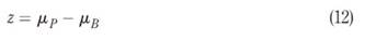
1. Introduction

Within the asset management sector, tracking error (TE) is a fundamental performance evaluation measure that has been used by the industry to ensure portfolio managers adhere to their given investment policy statement (IPS). TE is an active risk measure that stipulates the standard deviation of the difference between the portfolio return and the benchmark return (or excess return). In practice, TE gauges how consistently a portfolio outperforms or underperforms its designated benchmark, and it is used in conjunction with several other metrics to evaluate a portfolio’s performance, such as the value at risk and information ratio. Generally, TE results from security selection, taxes, factor tilts, transaction costs, cash management and general market volatility (^{Thomas et al., 2013}).

Portfolio managers pursue positive returns that are above the benchmark, while simultaneously adhering to mandated constraints as they have an incentive to outperform the benchmark to earn additional revenue from performance fees. Investors thus enforce a TE constraint, but this can result in portfolio managers focusing only on optimising excess returns and ignoring an investor’s overall portfolio risk (^{Roll, 1992}). TE is directly agnostic: it only determines the deviation of excess returns but articulates essentially nothing with regards to the direction of returns (e.g. positive or negative). Many investors incorrectly believe or assume that a higher TE is associated with a higher potential return, which may not always be true (^{Thomas et al., 2013}).

Other performance metrics such as the information ratio (a performance measure which does not account for total risk, only relative risk - see equation (1) - and is generally used ex-post performance) also ignores investors’ overall portfolio risk and exacerbate agency issues:

Higher information ratios could indicate higher excess returns but could also indicate an increase in absolute risk (^{Jorion, 1992}).

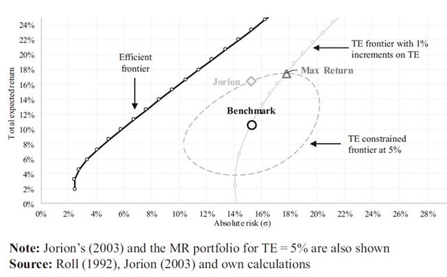
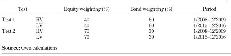
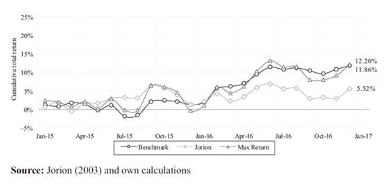
^{Jorion (2003}) developed a constant TE frontier which incorporated the risk of the benchmark. This frontier is an ellipse in mean/variance space, and which identifies a portfolio’s permissible return/risk profile given a TE constraint. Portfolio managers will ideally try to maximise the portfolio’s return, even if this incurs extra risk. This suggests that portfolio managers would essentially create a portfolio that lies on the uppermost point of this ellipse. However, Jorion’s (2003) suggestion of limiting the absolute risk of the portfolio to that of the benchmark would produce a portfolio with a lower coefficient of variation, thus optimising the portfolio in a mean-variance sense. Jorion (2003) noted that the shape of the ellipse was relatively flat; therefore, the reduction in expected return should be marginal. This article explores the effectiveness of Jorion’s (2003) proposal is in a practical situation by using a standard combination of equities and bonds in both bull and bear market conditions. The idea is to test, practically, whether investors would benefit from Jorion’s (2003) proposal, especially in challenging market conditions. Two periods are tested: a low volatility period (LV), to act as a basis for comparison and a high volatility period (HV) to represent a stressed market condition.

This article proceeds as follows: Section 2 presents the relevant literature and Section 3 introduces the variables and assumptions (e.g. transaction costs, rebalancing periods, asset weights, periods and TE constraint) which are required. The empirical results and discussion follow in Section 4 and Section 5 concludes the paper.

2. Literature review

Most asset managers are evaluated by their total return performance relative to a given benchmark, for example, the S&P 500. This leads to monthly performance reviews, in which portfolio managers and investors assess total returns after fees/expenses and compare these results to the allocated benchmark. Positive returns above benchmark returns (after fees/expenses) generally lead to the retention of the portfolio manager. Many investors thus focus on fund outperformance over the benchmark, which consistently results in positive expected TE. Unfortunately, asset returns are generally noisy and require several months of return data before one can reliably measure the average portfolio performance, after which investors can make an educated decision on the statistical significance of the portfolio’s return and determine if the portfolio manager is adding value. When portfolios are initiated, overall performance is not necessarily used, plus performance fees incentivise portfolio managers to take on additional risk to earn a higher return, which further detracts investors from focusing on the initial overall performance figure. This, in turn, causes investors to focus heavily on TE because a lower TE indicates fewer months of excessive negative returns, but also fewer months of excessive positive returns (^{Roll, 1992}).

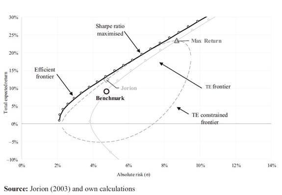
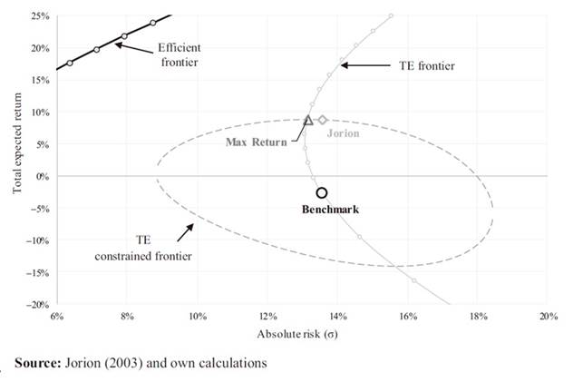
^{Roll (1992}) argued that a portfolio manager’s objective of outperforming the benchmark, while simultaneously attempting to reduce the portfolio’s TE, was comparable to the typical Markowitz mean-variance objectives with modifications. Roll’s (1992) work established the TE-constrained frontier - the locus of points in mean/risk space which represents the maximum return (MR) (and associated risk) for each level of TE (grey line in Figure 1). ^{Jorion (2003}) extended Roll’s (1992) work and derived a constant TE frontier - the locus of points in return/risk space which represent all combinations of return and risk for a given TE. The shape of the ellipse led Jorion (2003) to propose the extra constraint that portfolio managers observe the TE and match the portfolio risk (σP) to that of the benchmark (σB) i.e. that σP = σB. TE frontiers are not necessarily efficient.

Figure 1 Various frontiers 

^{Jorion (2003}) accepted the TE constraint as given, even though it is not optimal, as the TE constraint is widely used within the asset management industry and found that limiting a portfolio’s absolute risk to that of the benchmark, substantially improved portfolio performance.

^{El-Hassan and Kofman (2003}) explored the impact of inefficient benchmarks - which ^{Jorion (2003}) excludes - and introduced a short-selling constraint. Australian stocks were used during a period characterised by a strong bull market, followed by a severe, long bear market. El-Hassan and Kofman (2003) concluded that a short-selling constraint on a portfolio that exhibited Jorion’s (2003) absolute risk constraint caused the unrestricted weights to form entirely impractical values throughout the bear market conditions with considerable short-selling repercussions. The opportunity set was thus severely reduced, leading to constant rebalancing to maintain control over total risk in actively managed portfolios (^{Plaxco and Arnott, 2002}). This, in turn, meant that a short-selling constraint changes an actively managed portfolio into more of a passively managed portfolio (El-Hassan and Kofman, 2003).

^{Bertrand (2009}) extended the work of Bertrand et al. (2001) by creating portfolios in which the TE varied, but risk aversion remained fixed. These portfolios would then lie on what Bertrand et al. (2001) called an iso-aversion frontier. Bertrand (2009) demonstrated that optimal portfolios, which lay on the iso-aversion frontier had many desirable properties for portfolio managers, most importantly, all portfolios had the same information ratio. Portfolios that lay on this frontier had β < 1, so if portfolio managers embed their decision around the information ratio, there is minimal incentive to produce portfolios that would move away from the benchmark. As the absolute risk of the portfolio is identical to the total risk of the benchmark, taking on additional absolute risk would not incentivise a portfolio manager to create a portfolio that lies further away from the benchmark. Bertrand (2009) thus recommended portfolios that lay on the iso-aversion frontier, as these exhibit less risk than the benchmark while simultaneously dominating the benchmark in a mean-variance sense (Bertrand, 2009).

^{Bertrand (2010}) noted that performance attribution alone was inadequate and misleading. Volatility is also insufficient because of asset correlations. Bertrand’s (2010) study examines the information ratio breakdown suggested by ^{Menchero (2007}) with regards to the analysis of risk-adjusted performance attribution developed by Bertrand (2005). Bertrand (2009) showed that optimising portfolios only with a TE constraint was like the risk-adjusted performance attribution process proposed by Menchero (2007). If extra constraints (for example on total risk) are introduced, component information ratios would no longer be uniform; furthermore, they would not be equal to the information ratio of the entire portfolio. Equilibrium between the expected return and relative risk could not be attained (Bertrand, 2009).

^{Bertrand (2010}) found that increasing TE tended to decrease the information ratio. This showed that the additional TE allowance was not compensated for by additional returns. Forming a decision based solely on the information ratio alone meant that portfolio managers would have no incentive to produce portfolios that strayed from the benchmark, as σP = σB. Consequently, portfolio managers were not compensated for taking on additional risk, which Bertrand (2010) found disturbing.

^{Stowe (2014}) ascertained that portfolio managers optimise TE rather than standard deviation causes portfolio managers to optimise utility functions (parameterised in TE rather than invariance). Maximising utility is reliant on the interaction of the TE frontier with the principal’s given utility function. If the principal has “good enough” information, Stowe (2014) showed that a principal might be able to optimise the degree of the TE constraint (given quadratic utility), by enforcing an optimal TE constraint. In so doing, utility maximisation, given the delegated performance incentive, could be achieved. Therefore, Stowe (2014) also showed that the TE constraint is fundamentally a risk aversion constraint (Stowe, 2014).

^{Stowe (2014}) also discussed ^{Roll’s (1992}) conventional β constraints and found that having a β constraint in line with the principal’s level of risk aversion will always have a positive utility improvement for the principal (Stowe, 2014). This level of risk aversion is generally equal to the principal’s global optimal portfolio, so given the TE and β constraints, the portfolio manager is more likely to purchase the principle’s global optimal portfolio (Stowe, 2014).

The literature, then, largely overlooks absolute portfolio risk. It does not elaborate on these constraints with regards to real-world assets and differing periods. Much of the work has been theoretical, which may not be beneficial in a practical setting.

3. Methodology

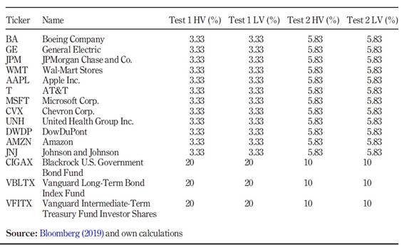
^{Jorion’s (2003}) proposal was evaluated using 15 different US-denominated assets assessed over two periods of differing market volatility.

3.1 Assumptions

The following assumptions were made

transaction costs/rebalancing costs - ignored;

regulatory constraints/tax constraints - ignored;

TE - held constant at 5%;

risk-free rate - held constant at 2.5% (to replicate the average yield on the 10-year Generic US Government Bond);

net short selling allowed - no limit on the degree to which an asset can be shorted, if the portfolio’s total weighting is 100%; and

portfolios are rebalanced monthly, as ^{El-Hassan and Kofman (2003}) maintained that constant rebalancing was required to maintain control of total risk. Daily rebalancing would more than likely require significant transaction costs and quarterly or semi-annual weightings would be insufficient to maintain control of total risk. El-Hassan and Kofman (2003) propose that at least monthly rebalancing is required to control both risk to a reasonable degree and keep transaction costs relatively low (even though transaction costs are ignored) (El-Hassan and Kofman, 2003).

3.2 Data

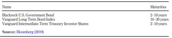
Adjusted data are used for these 15 assets: stock splits, dividends and share repurchase are all accounted for. Bond funds were chosen as this eliminates the need to constantly revalue positions, while simultaneously providing a traceable metric, as the funds trade similarly to equities. This simplifies the rebalancing of the portfolio assets.

The idea is only to test which of the ^{Jorion’s (2003}) benchmark risk portfolio (JB) and the MR portfolio generates superior returns in comparison to the benchmark, over different periods of market volatility.

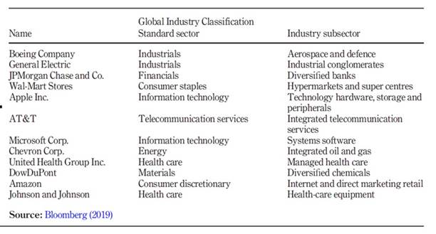
3.3 Asset selection

Tables 1 and 2 define the asset selection.

Table 1 Equity selection 

Table 2 Bond selection 

3.4 Testing methodology

Two years of historical data are used to determine the portfolio weights. Thus, the weightings for January 2008 are determined using January 2006 to December 2007 data. The following steps are involved:

Calculate the covariance matrix between all 15 assets using data from the previous two years (e.g. if calculating July 2008 weightings, one uses data from July 2006 to June 2008).

Calculate the average expected return for all 15 assets using data from the previous two years (again, for July 2008 weightings, data from July 2006 to June 2008 are used).

Use the two-year roll average covariance matrix and expected return data into ^{Jorion’s (2003}) formulas provided below to calculate a desired month’s weightings.

Record the monthly weightings for each portfolio, this being the benchmark portfolio, JB and MR portfolio.

Calculate the monthly weightings of the benchmark, JB and MR portfolio by the monthly returns for each asset until two years of data have been recorded.

Repeat the steps above until data for every two-year period is reached (this being four tests in total).

3.5 Time periods

Two different periods were examined.

3.5.1 Low volatility period - January 2015-December 2016.

This period was chosen because of the low VIX (Chicago Board Options Exchange volatility index) index values/volatility (average 17%) over the period from January 15 to December 16) in 2013 and 2014 (Figure 2). This LV was after the 2008 financial crash, post the sovereign crisis of 2011-2012. Post-2012, banks were well capitalised and oil prices and interest rates were relatively low, which encouraged both consumer and corporate spending, leading to growth. This, in turn, ensured global economic stability and low volatility (MCSI, 2012).

Figure 2 VIX index 

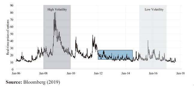
3.5.2 High volatility period - January 2008-December 2009.

This period was chosen because of the 2008 financial crash which caused considerable volatility (average 54% over the period from January 2008 to December 2009), as seen by the VIX index in Figure 2. This was largely caused by the subprime mortgage crisis which originated in 2007, followed by the collapse of Lehman Brothers on 15 September 2008.

3.6 Weightings

Initially, the weightings are set to those of a traditional portfolio, entailing that the portfolio comprises 40% equities and 60% bonds (Test 1). Within each asset class, the benchmark portfolio is equally weighted (Tables 3 and Table 4). Test 2 covers a portfolio more heavily weighted towards equities, i.e. 70% equities and 30% bonds.

Table 3 Benchmark weightings 

Table 4.Benchmark weightings expanded 

3.7 ^{Jorion’s (2003}) benchmark risk portfolio weighting calculations

To continue with the interpretation of the ^{Jorion (2003}) proposal, certain definitions are necessary.

q: vector of benchmark weights for a sample of N assets;

x: vector of deviations from the benchmark;

qP (= q + x): vector of portfolio weights;

E: vector of expected returns; and

V: covariance matrix of asset returns.

This work assumes that short selling is permitted to preserve linearity; therefore, the total active weight qi + xi may be negative for any specific asset. In general, the benchmark will have a positive weight; hence, the universe of assets can surpass the components of the benchmark; however, the assets that are used in the benchmark need to be included.

Expected returns and variances can now be expressed in matrix notation as:

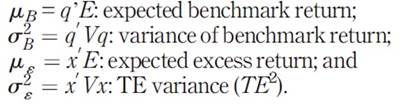
These are measures of risk and return that are forward looking, because x signifies current deviations and V the best estimation of the covariance matrix.

Therefore, the TE variance can be written as:

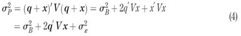
After this, one can stipulate the expected return and variance of the active portfolio as:

Constraint: portfolio needs to be fully capitalised, defined as:

where 1 represents an N-dimensional vector of 1 s.

Furthermore, using ^{Merton (1972}) calculations, the following variables are also defined: The outline of the constant TE volatility frontier with regards to the initial mean-variance space is defined by ^{Jorion (2003}) as:

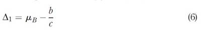
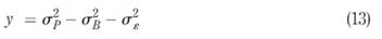
whereb/c= ^_μMV and

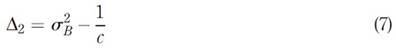
where ,which characterises both the expected return and variance of the index in excess of the return and variance of the minimum variance portfolio (with both Δ1 and Δ2 being positive).

3.7.1 Mean-variance frontier in the absolute return space.

Minimise subject to and with G being the target return.

To determine the vector of portfolio weights, the following formula is used:

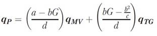
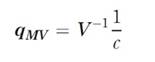
where qMV is the vector of asset weights for the minimum variance portfolio given by:

and qTG is the vector of asset weights for the tangent (optimal) portfolio given by:

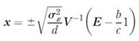
3.7.2 Tracking error frontier.

Maximise x′E subject to x′1 = 0 and . The solution for the vector of deviations from the benchmark, x, is:

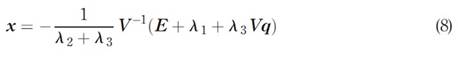
3.7.3 Constant tracking error frontier.

Maximise x′E subject to x′1 = 0, and . From here, the answer for the vector of deviations from the benchmark, x, is:

where:

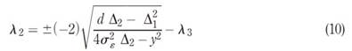
^{Jorion (2003}) defined

And

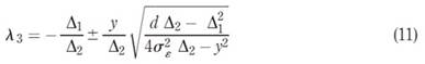
and established that the relationship between y and z is:

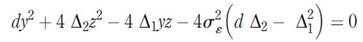
which is a quadratic equation in both y and z (^{Jorion, 2003}).

Solving for z:

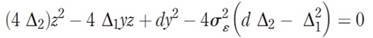
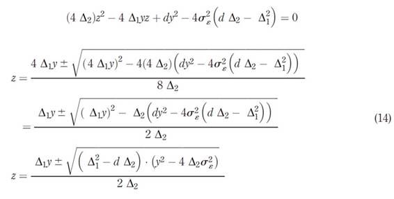
This describes the constant TE ellipse. ^{Jorion's (2003}) proposal of constraining the portfolio risk to that of the benchmark implies that 2q´ Vx = [from equation (3)].

4. Empirical results

4.1 Low volatility period (2015-2016)

The LV was included as a base measure or comparison measure. Hence, the initial hypothesis stated that the JB will not outperform the MR portfolio with regards to total return. This proved to be accurate throughout our testing with regards to the LV.

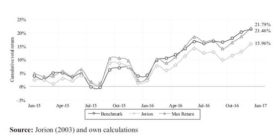
4.1.1 Total return.

There are several important conclusions to be drawn from these tests within the LV. First, the JB underperforms the benchmark in both Tests 1 and 2, when examining the total return figures over the two-year period (seen in Figures 3).and 4 ). This makes the JB a less attractive option during LV, especially when considering transaction costs. In both tests, the MR portfolio only marginally outperformed the benchmark portfolio and if transaction costs were included, it possibly would have underperformed the benchmark portfolio. Hence, given the LV and the assets used, an enhanced return by passively investing in the benchmark portfolio is expected.

Figure 3 Cumulative return, Test 1, low volatility (40%equities and 60% bonds) 

Figure 4 Cumulative return, Test 2, low volatility (70%equities and 30% bonds) 

4.1.2 Mean-variance return.

In a mean-variance sense, the JB exhibited a lower coefficient of variation (σ/µ) in comparison to the MR portfolio for essentially the whole two-year LV (except for January 2015 to March 2015 in Test 1 LV). In Test 2 LV, the JB exhibited a lower coefficient of variation throughout the whole two-year period.

4.1.3 Benchmark efficiency.

The proximity of the JB to the efficient frontier could be because of a comparatively efficient benchmark, thus the benchmark weightings in the LV are close to the optimal weights of the efficient frontier. This is further supported by ^{Jorion (2003}), who maintains that a portfolio with an absolute risk constraint will achieve a superior mean adjusted return, given that the benchmark is inefficient. The point at which the TE constrained frontier touches the efficient frontier is the point at which the Sharpe ratio is maximised. An interesting avenue for future research could compare a portfolio with a maximised Sharpe ratio to the JB or MR portfolio, given a TE constraint and an efficient benchmark. This was recently explored by ^{Maxwell et al. (2018})( Figures 5 and 6 ).

Figure 5 Monthly return difference between JB and MR portfolios, Test 1, low volatility 

Figure 6 Monthly return difference between JB and MR portfolios, Test 2, low volatility 

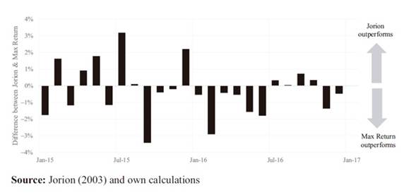
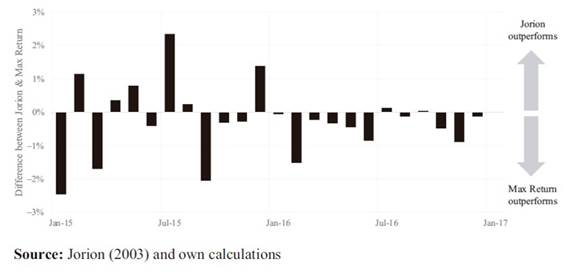
Figure 7 is a snapshot of January 2015’s expected return and absolute risk, obtained from the two-year rolling average. The values in Figure 7 represent the average expected return and absolute risk that was achieved in the two years before January 2015. This period was chosen as the difference between the JB’s absolute risk and the MR portfolio’s absolute risk is at its greatest, at a difference of −3.96%.

Figure 7 Test 1, low volatility, January 2015 

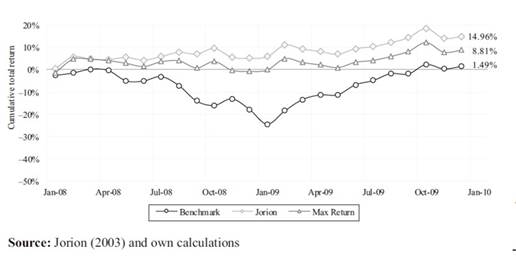
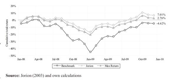
4.2 4.2 High volatility period (2008-2009)

Moving on to the HV, Figures 8 and 9 show that the results are significantly different from that of the LV. The JB portfolio outperforms the MR portfolio in the two-year period and more importantly, the JB significantly outperforms in August and September 2008, which one could say was fundamentally the start of the 2008 financial crisis with Lehman Brothers filing for bankruptcy on 15 September 2008. The JB in Test 2 HV outperformed the MR portfolio in October 2008, which saw some of the largest losses in the S&P 500 and experienced one of the highest VIX index values seen to date.

Figure 8 Cumulative return, Test 2, high volatility (40%equities and 60% bonds) 

Figure 9 Cumulative return, Test 2, high volatility (70%equities and 30% bonds) 

4.2.1 Total return.

Test 1 HV produced a superior total return to Test 2 HV, both in terms of total return and the difference between ^{Jorion (2003}) and the MR portfolio. Compared to the LV, Test 2 LV portfolio outperformed Test 1 LV portfolio (both in terms of the total return and the difference between JB and MR).

Portfolios that use benchmarks with higher bond weightings should theoretically outperform portfolios with heavier equity weightings in HV. In LV, the opposite is true.

This is intuitively appealing because in periods of financial distress, investors would demand safer investments, which in this case could have caused an increase in demand for the Vanguard Intermediate-Term Treasury Fund (VFITX) fund from the JB. Furthermore, the US 10-year treasury yields decrease substantially in late 2008, further emphasising the increase in demand for safer assets in the financial crash (^{Hall, 2010}).

4.2.2 Tracking error constrained frontier.

JB’s portfolio exhibits a higher absolute risk value than that of the MR portfolio (given that this only occurs from December 2008 to December 2009 - Figure 12 ). JB exhibits higher volatility than that of the MR portfolio in both Tests 1 and 2; hence, the JB inverts positions with the MR portfolio when compared to the LV. This could be because of an inefficient benchmark, which not only exhibits a weaker expected return, but also a higher absolute risk value in comparison to the MR portfolio. Further emphasis can be gathered from Figure 12, as the benchmark portfolio is further down the TE frontier curve in comparison to the LV. Furthermore, the MR portfolio will always lie on the uppermost point of the TE frontier ellipse; therefore, the shape of the ellipse in the HV is flattening and possibly shifting leftward, which decreases the potential return for the MR portfolio.

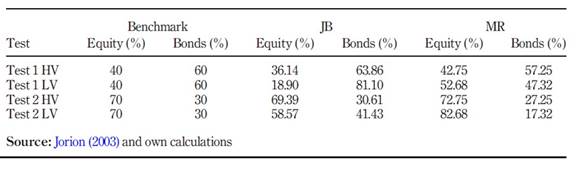
4.2.3 Portfolio weightings.

Following on from Section 4.2.2, one can see how asset weights deviate between each portfolio over the two-year period, hence causing the JB and MR portfolio to invert.

From Table 5 there is a significant deviation from the benchmark weightings with regards to the LV, especially with regards to the JB in Test 1 LV and the MR portfolio in Test 2 LV. This seems to suggest that equities in the LV are not suitable for the JB because of higher absolute volatility in equities and the comparatively lower allowable absolute risk, given the benchmark’s absolute risk. In the HV, the JB is not constrained as excessively, as the absolute volatility of the benchmark rises, thus enabling the JB to select higher returning and riskier assets. This was also found by ^{Jorion (2003}) who argued that his proposal is beneficial if the benchmark is inefficient relative to the efficient frontier (^{Jorion 2003} ).

Table 5 Average portfolio weightings 

This creates a curious dynamic in Test 1 HV, as the VFITX bond fund becomes grossly overweighted to roughly 311% in February and March of 2008. This dynamic was noted by ^{El-Hassan y Kofman (2003}), who maintained a short-selling constraint in their portfolio while adhering to ^{Jorion (2003}) absolute risk constraint. Therefore, in Test 1 HV, the JB would not be attainable if such a short-selling constraint is present, as then the 311% weighting in the VFITX bond fund could not be offset by short-selling other assets (^{El-Hassan y Kofman, 2003} ).

4.2.4 Standard deviation of the monthly ^{Jorion (2003}) returns.

Upon further examination, the standard deviation of the monthly returns is clearly lower than that of the monthly benchmark portfolio and marginally lower than the monthly MR portfolio. This is interesting as the LV did not produce a similar result. In the LV, the benchmark portfolio clearly exhibited a lower overall monthly standard deviation than that of the JB and MR portfolio. This indicates that the JB exhibited a lower degree of volatility concerning monthly returns than both the benchmark and the MR portfolio, with the benchmark portfolio exhibiting the largest degree of monthly return volatility among the three portfolios in the HV. This was supported by both ^{Roll (1992}) and ^{Grinold (1992}), who stated that most benchmarks were inefficient when compared to the efficient frontier (^{Grinold (1992})( Figures 10 and 11 ).

Figure 10 Monthly return difference between JB and MR portfolios,Test 1, high volatile 

Figure 11 Monthly return difference between JB and MR portfolios, Test 2, high volatilityty 

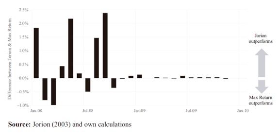
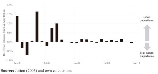
Figure 12 represents July 2009, as the difference between the JB’s absolute risk and the MR portfolio’s absolute risk is at its greatest, at a difference of 0.41%. As before, the values in Figure 12 represent the average expected return and absolute risk that was achieved in the two years before July 2009.

Figure 12 Test 1, high volatility, July 2009 

5. Conclusions and suggestions for further study

Active portfolio managers are bound by TE constraints, which ignore absolute risk focusing instead on excess return optimisation, which generally increases total portfolio risk in LV. ^{Jorion (2003}) showed that a TE constraint leads to an ellipse around the benchmark of attainable portfolios, given the portfolio meets the IPS. Hence, ^{Jorion (2003}) found that limiting absolute risk to that of the benchmark can be advantageous in a mean-variance sense if there are relatively low admissible levels for TE or if the benchmark is inefficient.

^{Jorion's (2003}) constraint on absolute volatility is beneficial in HV, such as the 2008 financial crash, due mainly to an inefficient benchmark (given the HV), which allowed the JB to exhibit both higher absolute risk and expected return values than that of the MR portfolio. This is significant as the MR portfolio traditionally outperforms the JB with regards to total return in LV, as the MR portfolio attempts to optimise excess returns by achieving the maximum possible return given the TE constraint, as seen in Figure 1. Hence, the MR portfolio is always situated on the uppermost portion of the TE ellipse and is generally not efficient when compared to the JB. In a HV, the JB and MR portfolios invert positions to a relative degree, thus making JB more desirable.

In the HV, the JB heavily favours bonds, especially from January 2008 to August 2008. For example, the JB heavily favoured the VFITX in January 2008 to August 2008 period, especially when the benchmark exhibited a higher weighting for bonds (as seen in the Test 1 HV results). However, this is relatively realistic given that demand for safer assets increases in times of financial instability (^{Hall, 2010} ).

In LV, the JB is unattractive: it underperforms the benchmark considerably (especially if transaction costs are considered). However, the JB was still more efficient in a mean-variance sense. The MR portfolio marginally outperformed the benchmark in the LV and surely would have underperformed the benchmark if transaction costs were considered. This was ultimately because of a relatively efficient benchmark, as the benchmark lies closer to the efficient frontier in comparison to the HV. This affirms ^{Jorion (2003}) conclusion that a constraint on absolute risk is beneficial when inefficient benchmarks are present.

Future studies could include transaction costs to ascertain whether an actively or passively managed strategy would be advantageous, especially in LV. Additional assets could also be added, both with varying degrees of benchmark efficiency and differing benchmarks. Additional assets or asset classes could improve results with regards to ^{Jorion (2003}) proposal, especially if the chosen assets form an inefficient benchmark, or low levels of admissible TE volatility are present.

Creating a portfolio which maximises the Sharpe ratio in periods of low volatility, when a relatively efficient benchmark is present, creates a portfolio that lies on the efficient frontier. ^{Maxwell y col. (2018}) found that maximising a portfolio’s Sharpe ratio can provide certain desirable results. Comparing a portfolio with a maximised Sharpe ratio to the JB or MR portfolios, given a TE constraint, might lead to an interesting outcome in both HV and LV.

In LV, ^{Jorion's (2003}) constraint on absolute risk is counterproductive, especially if the benchmark is relatively efficient and one is solely focusing on total return. Whereas, in a HV, the ^{Jorion's (2003} constraint can be beneficial, given the benchmark is relatively inefficient.