


 Inglés (pdf)
 Articulo en XML
 Referencias del artículo
 Enviar articulo por email
 Citado por SciELO
  Similares en
SciELO
Similares en
SciELO 
 Permalink
Introduction
Authors such as Trigeorgis (1996), Mun (2002) and Damodaran (2019) recognize there is a difference between the theoretical concepts of valuation of capital assets and their empirical approximation, a discrepancy that is reflected in a gap not deeply explained and with sufficient academic rigour between the market value and its theoretical estimate. Therefore, different methodological alternatives have been proposed to mitigate this difference, but few consider key factors that generate value, such as those that try to measure and estimate uncertainty through the use of volatility, which usually has been moderately studied and ends up being relevant at the moment of making any type of valuation on a capital asset (Dixit and Pindyck, 1994; Valencia Herrera and Martınez Gandara, 2009; Alvarez Echeverra, et al., 2012).
In academia, the use of discounted cash flow (DCF) as a method used to value capital assets is common, but there are numerous criticisms about its use because it does not include elements such as contingent events, risk present in the cash flows and volatility (Trigeorgis, 1996). To overcome some of these problems, the real options approach (ROA) was developed, which complements the DCF and allows it to include volatility as a fundamental parameter to quantify the risk and collect some elements associated with uncertainty (Keswani and Shackleton, 2006; Sabet and Heaney, 2017). The ROA model was derived from its simile in the theory of financial options by modelling the value of assets as a call or put options, considering that it is applied to investments in assets or real markets, although there is not a tradable market (Cobb and Charnes, 2004).
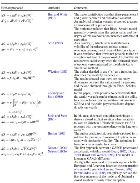
Since the Black and Scholes’s (1973) seminal work, which is considered generally used as a method for estimating the value of European call and put options, multiple models and extensions have appeared that allow the valuation of other types of options in different contexts, using of different estimation techniques, such as closed analytical solutions, finite difference method, Adomian decomposition method and numerical method through multiplicative and additive binomial trees, but the problem of considering volatility constant persists. Recently, some models have appeared to include stochastic volatility and were created, fundamentally, to avoid considering this fixed variable in terms of evaluation time horizon. Motivated by this empirical evidence, several authors, such as Hull and White (1987), Scott (1987), Scott (1987), Chesney and Scott (1989), Stein and Stein (1991) and Heston (1993), have proposed models that involve stochastic volatility as a parsimonious extension of the Black-Scholes model (Black and Scholes’s (1973). Amongst previously mentioned models, the GARCH-diffusion type proposed by Drost and Werker (1996), Duan (1997) and Duan(1996)offers the first approximation between a GARCH process and a stochastic volatility model, supported by multiple research theoretical (Ritchken and Trevor, 1999; Barone-Adesi et al., 2005; Christoffersen et al., 2010; Chourdakis and Dotsis, 2011) as well as empirical (Figa-Talamanca, 2009; Plienpanich et al., 2009; Wu et al., 2012, 2014, 2018). This paper proposes and motivates the inclusion of stochastic volatility in the ROA model, considering a rigorous mathematical development from a GARCH-diffusion stochastic differential equation (SDE) that has a numerical solution using multiplicative trees; besides, a prior estimate of a GARCH (1,1) process is required to allow an adequate real options valuation in real-world and risk-neutral situations. This paper is organized as follows: Section 2 summarizes the stochastic volatility models and describes the GARCH-diffusion model used for the development of this research. Section 3 presents, in summary, the multiplicative quadrinomial tree method to assess real options. Section 4 offers a brief description of real options valuation, specifically, its use according to the method proposed. In Section 5, we present a series of numerical experiments and some examples. Finally, Section 6 is the discussion and conclusions.
2. Literature review
One of the strongest assumptions considered in the Black-Scholes model (Black and Scholes, 1973) is that volatility ðσÞ is constant; many studies have demonstrated that logarithm of returns on asset prices have leptokurtosis and conditional variance that changes randomly as a function of time (Grajales Correa and Perez Ramırez, 2008) and the assumption of conceiving a normal distribution does not apply (Fernandez Castano, 2007 ~ ), additionally, implied volatilities are considered non-constant and differ between exercise prices and time to maturity. For these reasons, several extensions have been proposed in the literature in which volatility is considered a function of time as well as the price of the underlying asset, whereupon the linearity of drift and diffusion components of the asset price are maintained but incorporate a second equation that allows modelling the variance behaviour of St.
2.1 Stochastic volatility models
A model with stochastic volatility describes its change over time and generalizes the Black- Scholes model, defined in a given filtered probability space (Ω, F , F t, ℙ), which generally satisfies a system of SDEs (Hull and White, 1987; Scott, 1987; Wiggins, 1987; Chesney and Scott, 1989; Nelson, 1990 a, Nelson, 1990b; Stein and Stein, 1991; Heston, 1993; Hilliard and Schwartz, 1996; Drost and Werker, 1996; Duan, 1996, 1997; Wilmott, 1998; Ritchken and Trevor, 1999; Barone-Adesi et al., 2005; Chang and Fu, 2009; Figa-Talamanca, 2009; Moretto et al., 2010; Christoffersen et al., 2010; Chourdakis and Dotsis, 2011; Wu et al., 2012; Wu et al., 2014; Wu and Zhou, 2016; Peng and Peng, 2016; Wu et al., 2018; Wu et al., 2020, see Table 1). We considered an SDE system described as follows:
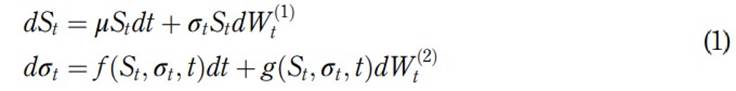
where μ is constant and volatility σt is considered as a dynamic variable in the price St. Studies like Wu et al. (2018) showed that the implied volatility, captured from historical data from the market, takes a relevant role in fitting the prices of the options asKim and Ryu (2015) explained as well. Functions f and g correspond to the tendency and diffusion of volatility, respectively. The model incorporates two sources of randomness W t (1) and W t (2) that correspond to Wiener’s standard processes with a correlation coefficient ρ. The price process {St; 0≤t ≤T} is not completely described by equation (1), and the value St will be conditioned to the information of S0, σ0 and to the trajectory followed by volatility {σs; 0≤s≤t}.
The GARCH-diffusion model was introduced by Wong in 1964, but its popularity only grew following the works of Nelson (1990 a, Nelson, 1990b). An important condition was discovered by Christoffersen et al. (2010) who demonstrated empirically, through the use of realized volatilities on the S&P500 returns with an option’s data panel, that the Heston model was poorly specified because, in the diffusion model presented by the author, volatility was found in the square root instead of being considered linear; these conclusions were reaffirmed by Chourdakis and Dotsis (2011) although they also suggested that the model should consider a nonlinear drift against a linear one.
Recent studies have indicated that this model allows a better description of the behaviour and dynamics of financial series than other types of models, such as Heston (1993), Aıt-Sahalia and Kimmel (2007), Jones (2003) and Wu et al. (2018). Also, it has been used as a good model for adjusting financial option data (Christoffersen et al., 2010; Chourdakis and Dotsis, 2011; Kaeck and Alexander, 2012; Wu et al., 2012, 2014, 2018, 2020).
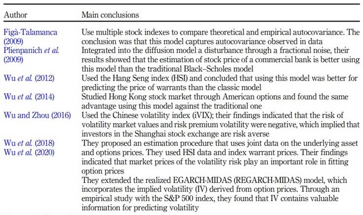
The most recent applied research related to this model is summarized in Table 2. In general terms, this type of model is usually characterized by not having a closed solution and is in the class of non-affine models; also, their solutions must be achieved with simulation, numerical methods (Wu et al., 2012) or the use of integrals in SDEs (Barone-Adesi et al., 2005; Florescu and Viens, 2008; Vellekoop and Nieuwenhuis, 2009). The system of traditional equations presented by this model has the following functional structure (Barone-Adesi et al., 2005):
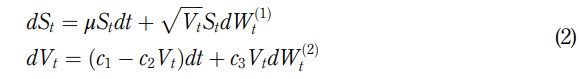
where c1, c2 and c3 are positive constants; μis the tendency parameter; c2 is the mean-reversion rate; (c1)/(c2) is the mean long-term variance and c3 models the random behaviour of volatility and corresponds usually to the volatility of volatility. For its part, W(1) t and W(2) t correspond to Wiener processes with a correlation coefficient ρ
An alternative way to present the structural form of equation (2) is an SDE; following (Wu et al., 2012):

Table 2 Summary of the empirical or applied research of GARCHdiffusion mode
Source(s): Own elaboration
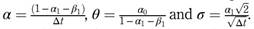
where parameters α, θ and σ are constant and are equivalent to the mean-reversion speed, the mean long-term volatility or tendency and the volatility of volatility, respectively. Consequently, W t (1) and W t (2) correspond to independent one-dimensional standard Wiener motion processes.
This paper focuses on using equations (3) and (4) to summarize the numerical method for a multiplicative quadrinomial tree that includes stochastic volatility, which will allow the valuation of a derivative instrument, such as real options, when the volatility of the underlying asset is stochastic. Hence, we use the equivalence proposed by Hull (2003) and described by others (Pareja-Vasseur et al., 2020) that relates the conditional variance from GARCH (1,1) and the stochastic variance from differential equation proposed in (4), i.e. Vt is equivalent to h2 t , with
These set of parameters of the conditional variance could be estimated by the maximum likelihood method, through computational tools such as Eviews or MatLab, previously checking the assumption of conditional heteroskedasticity (Bollerslev, 1986).

2.2 Quadrinomial recombination
The multiplicative quadrinomial trees methodology is summarized below, including all formulas for probabilities and transitions factors, and discounted rates. Considering the GARCH-diffusion model, over the time interval (ti; tk), where μ ∈ ℝ, α ≥0, θ > 0 and σ > 0 are constant, while {Wt (1)} t≥0 and {Wt (2)} t≥0 are independent one-dimensional standard Wiener motions, supposing further that St = Si and Vt = Vi, probabilities of the transition and growth factors for the processes Vt and St, respectively, are defined as Pareja-Vasseur and Marın-Sanchez (2019) and Marın Sanchez (2010
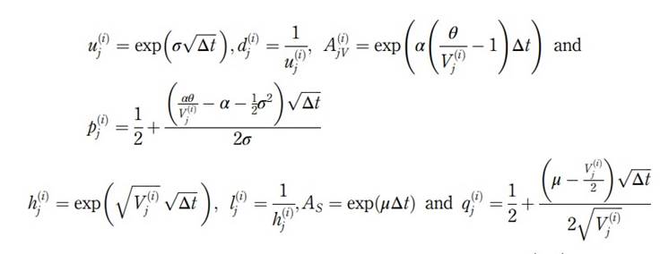
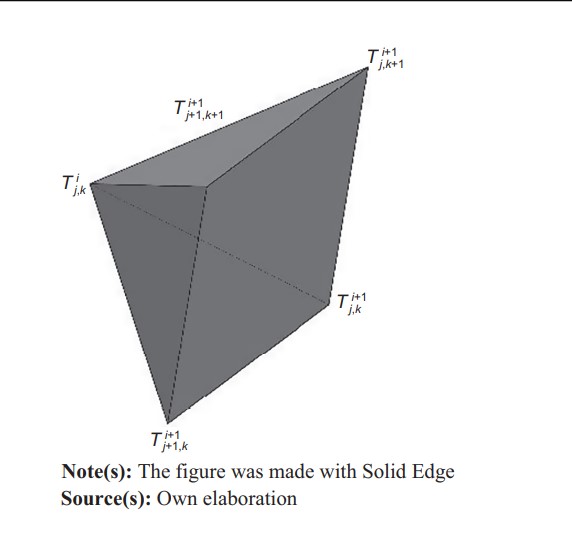
To consider the recombination of two binomial trees
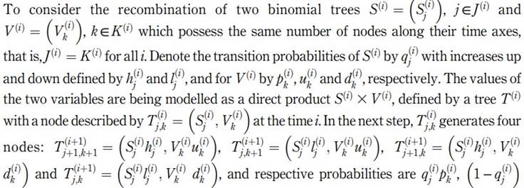
, respectively (Lari-Lavassani et al., 2001) (Pareja-Vasseur and Marín-Sánchez, 2019).
After all the corresponding parameters have been defined for Vt and for St, it is possible to construct a tree that emulates the behaviour of the price St, where each discrete step has a value of branches equal to 4n, where n corresponds to the number of steps, but when the respective recombination is performed, the number of branches decreases to n2 , as can be seen in Figure 1. Also, the value of each position for the first step of the tree is presented in Figure 1 (Pareja-Vasseur and Marín-Sánchez, 2019).
Method
It is common knowledge that an option is considered a financial instrument that grants a right to the buyer and an obligation to the seller, to buy or sell a certain asset or underlying asset at a price established on a fixed date; the exchange price that is obtained for acquiring the option is known as premium. Amongst the methods used in its valuation, the multiplicative binomial method is the most often used and appropriate because it is easy to understand and construct (Cox et al., 1979). After all, it allows us to emulate the price of the underlying asset in discrete time and offer the respective valuation of the derivative.
3.1 Real options valuation
One of the recent development techniques for valuing capital assets is known as ROA; according to this method, which is complementary to the DCF model, the aim is to introduce the volatility present in cash flows and the occurrence of contingent events. The method emerges from the theory of financial options, except the valuation is performed for capital assets in real markets. This type of options, such as financial options, can be assessed using different techniques, where the most appropriate is the numerical method with multiplicative binomial trees (Cox et al., 1979), because of its simple and intuitive handling, in the sense that continuous-time price of an underlying asset approximates to a geometric Brownian motion (GBM) (Smith, 2005; Sina and Guzmán, 2019), emulated through a process in discrete time organized as a tree, where it is possible to analyse, in graphical and numerical forms, the anticipated execution (or not) of the option. The ROA technique allows us to assess the strategic Net Present Value (NPV), through the appropriated estimation of the premium value of call/put options and comparing this value to the traditional DCF method, which is also called static NPV. According to this theory, options are used to, for example, defer, contract, expand or abandon that correspond to American call and put options adapted or modified to that context (Sabet and Heaney, 2017; Sina and Guzmán, 2019).
The main criticism of this methodology is that the same variables are used as in financial options valuation, with any kind of adjustment respect the application’s field. Specifically, the problem lies in these variables: the discount rate and volatility. The first problem concerns some adjustment measures, and it is even possible to use utility functions to represent an economic agent that models attitudes and preferences for a certain situation and thereby estimate the value as a true equivalent, using a risk-free discount rate without complications (Pareja Vasseur and Cadavid Perez, 2016). The second problem is the precarious development of the theoretical approaches to estimate volatility; the traditional estimation methodology, starting from the logarithmic return of the cash flows (Rogers, 2002) to the conditional volatility method of Brandao et al. (2012, going through the normal returns of cash flows (Lewis and Spurlock, 2004), the project proxy approach, the market asset disclaimer method or Copeland and Antikarov’s method (Copeland and Antikarov, 2003) the administrative estimates or made by experts, the correlated risk-free asset (Trigeorgis, 1996), the market proxy approach or historical analysis (Mun, 2002), the implied volatility ((Lewis and Spurlock, 2004), the Herath and Parks method (Herath and Park, 2002) and those of Godinho (2006), basically focused on the estimation of the unconditional volatility, which retains the drawback of assuming this phenomenon as constant. Works such as Brandao et al. (2012 only allow us to estimate it conditionally but without exploring the benefits of modelling it stochastically.
Most of the volatility estimation methods based on the ROA technique are basic, built on a single-level SDE, which only allows modelling the random asset’s price, and fails to include the effect of volatility on this variable. A differential equation that commonly uses the following structure is given by:

with t ∈(0;T) and the initial condition S0 = St, where μ is constant and denotes the asset’s average rate of return, σ > 0 corresponds to volatility and {Wt} t≥0 is a one-dimensional standard Wiener process.
Because of that it is necessary to make progress on both sides: the estimation of the volatility phenomena and its respective modelling through numerical methods because the high number of methodologies focuses mainly on an unconditional estimation of it. Finally, some of these techniques only present basic models for estimating the variable treated, which allows more advanced extensions or versions to be modelled, both the underlying asset and the volatility behaviour, conditionally and stochastically, but none of them explore the necessary changes that must be implemented in the valuation of options with these methods, specifically numerical ones, which are the most used and are also a motivation for the current research.
3.2 Algebraic expression
Assume an option (real or financial) over an asset that does not pay dividends, with an initial price S0 and strike price K, is divided into N sub-intervals, each one with duration Δt. Define f(i) j;k the value of the option in the node (i; j; k). Based on Marın Sanchez (2010) and (Pareja Vasseur and Cadavid Perez, 2016, the price of the asset has quadrinomial recombination in node (i; j; k), which can be represented by the following expression:
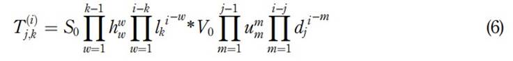
with T0 = T (1) 1;1 ; i = 2; ... ;N, j = 1; 2; ... ; i and k = 1; 2; ... ; i. Keep in mind that in this case, both u and d are constant, so equation (6) can be summarized as follows:

Below there is an algebraic approach based on the proposed methodology to assess the basic real options:
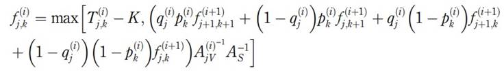
(1) In case of an option to wait, the evaluation is performed in a similar way as the American financial call option - where the value at its maturity date is given by maxðTt − KÞ; so,
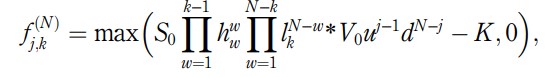
for j = 1; 2; ... ; i and k = 1; 2; ... ; i., while its discounted value is defined as
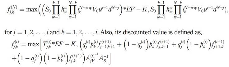
(2) In case of an expansion option, where the expansion factor is defined by EF and K represents the additional investment for expansion, it is considered as a modified American call option and the value at its maturity date is given by max(Tt*EF − K;Tt); so,
(3) In case of a contraction option, the contraction factor is defined by CF, and at the same time, K represents the disinvestment or release of funds by contraction, it is considered as a modified American put option and the value at its maturity date is given by max(Tt;Tt*CF + K); so,
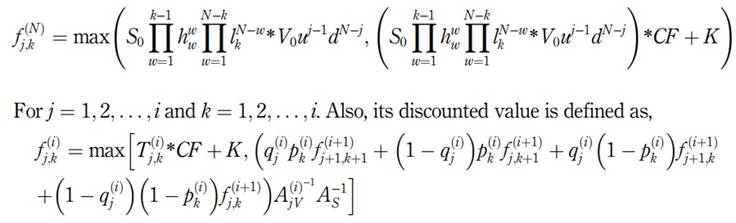
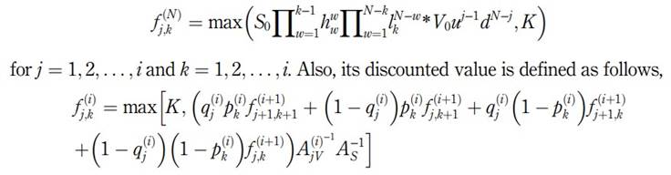
(4) In case of an abandonment option, the salvage value corresponds to K, it is considered as a modified American put option, the value at its maturity date is given by maxðTt; KÞ; so,
3.3 Risk-neutral valuation
To evaluate options in a risk-neutral world, two conditions must be assumed: The first is that estimated future cash flows can be determined by discounting their expected values at the risk-free rate, and the second is that the expected return on derivatives is the risk-free interest rate. To eliminate the potential for arbitrage on the discounted expected value, a single probability measure P* must be constructed from the subjective p, such that discounted price at interest rate r is a martingale and as mentioned earlier, the discounted expected value at this rate according to the new probability P* does not present arbitrage opportunities. The measure of the probability that is considered in a risk-neutral world is known as Martingale equivalent measure (MEM). Following Heston (1993), Marın Sanchez (2010), Pareja-Vasseur and Marın-Sanchez (2019), Wu et al. (2012), Wu et al. (2014) and Wu et al. (2018) and applying the theorem Cameron-Martin-Girsanov and Girsanov’s theorem (Mao, 1997, pp. 270-272), the discounted pay based on the risk-free rate r is S* t = e−rtSt and its stochastic differential corresponds to:
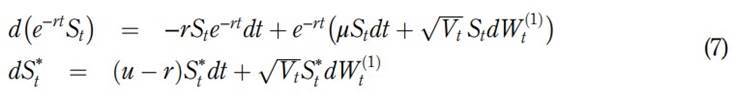
As above, the discounted price S* t satisfies the same equation that St, where the return μ had been replaced too (μ −r). This way the expected value under the subjective probability P from the discounted payoff of a derivative instrument will present arbitrage opportunities due S* t is not a Martingale. To find a probability measure where S* t is a Martingale, equation (7) must be written in a way that the tendency term could be assimilated inside the Martingale term. From there, the two previously mentioned theorems could establish that (μ−r) and
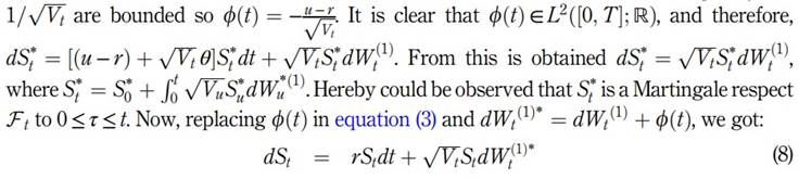
Note that equation (8) corresponds to the behaviour price in a risk-neutral world. In the same way to equation (4), the following expression is obtained:
that in terms of market risk premium associated with volatility, it could be represented by
accordingly to
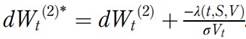
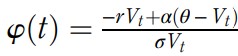
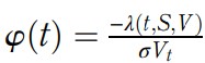
Substituting in equation (4) and considering that λ(t; S;V) is proportional to volatility, ∃ λ > 0 such as λ(t; S;V) = λVt, so
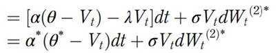
where α* = (α + λ) and θ* = θ αð/(α+λ) , {W(1) t*}t≥0 and {W(2) t*} t≥0 are independent onedimensional standard Brownian motions in the probability space (Ω, Ғ, P* ). The term λ(S;V; t) represents the price of volatility risk and is independent of the particular asset, and there is evidence that this term is not zero for options (Heston, 1993), while in contrast, Hull and White (1987) proposed to set this term at zero, based on the assumption that it is independent of the aggregate consumption. This term is the variance risk premium as a linear function of variance, namely λ(Vt; t) = λVt (Wu et al., 2012, (2014, (2018). Following Heston (1993) theory, this parameter should be determined for each particular asset (Pareja-Vasseur and Marın-Sanchez, 2019).
Results
4.1 Comparison between quadrinomial method with stochastic volatility, a binomial method with constant volatility and the Black-Scholes equation
Before presenting examples applying the proposed methodology using real options, it is necessary to graphically illustrate the asymptotic behaviour of quadrinomial and binomial methods, comparing the results with those obtained with the Black-Scholes model. Suppose that the dynamic behaviour of daily prices of a given financial asset can be modelled by a GBM, using equation (5) with an initial condition S0 = 10 and an annualized volatility σBS = 0:3162. Previous studies like Aziz (2017) assumed the historic price volatility capture properly the annual volatility project. With that in mind, now let us assume that it is required to value a European call finance option derived from the underlying asset, whose exercise price is K = 10, with risk-free rate r = 0:05 and time to maturity T = 1; likewise, consider traditional multiplicative recombination in binomial trees with N = 200. It is possible to verify that the binomial method is a particular or special case of the multiplicative quadrinomial when V0 = (σBS) 2 = θ and σ tends toward zero. Let us further assume that α is an arbitrary constant.
Figure 2 presents the results, showing that quadrinomial and binomial methods have near solutions at around N = 100, with values that are also proximate to those of the exact solution estimated by the Black-Scholes model. Based on the previous results, we can conclude that the traditional binomial tree is a particular case of the quadrinomial proposed model, indicating that our model is not just a generalization, but also more flexible to evaluate different contracts where the underlying asset does not necessarily behave like the classic GMB. Our framework opens a broad window to build analogous procedures with a different stochastic process (e.g. as could be Heston’s and Scott’s model), which are used on financial option valuations, and few studied on real options.
4.2 Example 1: valuation of an abandonment real option and sensitivitys analysis of the variables in the model in a real-world and risk-neutral world
Suppose that a firm in a certain sector of the economy wants to know the strategic value of a project according to ROA methodology and that its cash flows can be modelled using the SDE with equations (3) and (4). Assume in this case, the price of the commodity used to estimate the cash flows is perfectly correlated with a project, and its respective cash flows and volatility equal to the cash flows and the project’s volatility without administrative flexibility, as stated in Brandao et al. (2012). The estimated present value of the project is S0 = T0 = 100, which was estimated according to the traditional DCF methodology using an appropriate riskadjusted rate. The company also determined that it has an opportunity to assign the rights and property of the project to a third party at a value of K = 75 when the market conditions are unfavourable, that is, this value corresponds to the salvage value and remains constant
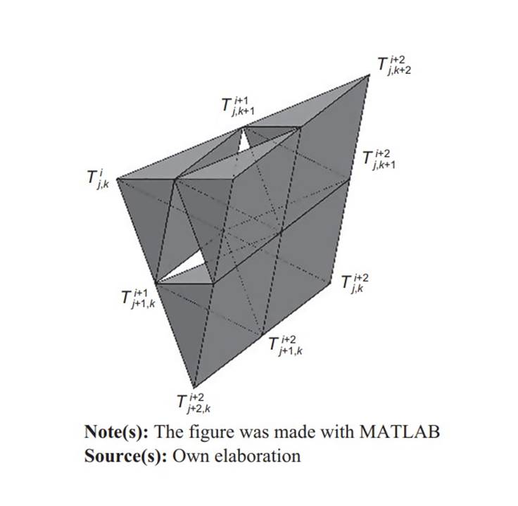
Figure 2 Comparison between quadrinomial proposed methodology, traditional binomial method and the Black- Scholes method
over the evaluation horizon of the firm’s abandonment option. Assume, besides, the following arbitrary values: V0 = 0:1, r = 0:05, α = 0:01, θ = 0:1 and σ = 0:1131, for the proposed method, and σBS = 0:3162 to the multiplicative binomial traditional methodology.
The results of the strategic NPV for the periods from Year 1-5, with steps of two years, are summarized in Table 3. Further, it was necessary to compare the results of the same methodologies, but in this case, the volatility σ tending towards zero was assumed for the proposed sample to show that it is a general case containing the particular one (caused by the traditional binomial method). In the last row of Table 3, we can see that the proposed methodology had a strategic NPV equals to 105:16, with a value of the abandonment option 5:16. If we assess them at three years, we found a result that was roughly in line with the traditional methodology, with 105:37 and 5:37, respectively. It was therefore concluded that there is a difference of less than 1% amongst the NPVs for the different evaluation periods presented. After estimating the volatility value of the volatility for the proposed method, the strategic NPV was set to a value of 108:51 for the case of σ = 0:1131, with the corresponding abandonment option corresponding to 8:51 if valued over five years. These results will increase depending on the different values estimated for parameters σ and α. It is worthy to mention that in this case, we are relaxing the constant volatility assumption, and due to the estimation of the quadrinomial tree, we can estimate properly the value of the option without this restriction. This means that a traditional estimation of an abandonment real option will be inadequately estimated, regardless it is under or overestimated.
4.3 Example 2: a valuation case of an abandonment real option in a real-world
This example describes a real options valuation case using the algebraic expression of an option of abandonment to find the value of the strategic NPV (the strategic NPV is the one estimated through the ROA, and it considers the static NPV calculated through the CDF, as the value of the real options identified and valued for a project). The numerical method utilized was our proposed methodology (a recombining quadrinomial tree with stochastic volatility and considering the values estimated for the proposed system). Finally, the solution was compared with the estimated results of the traditional binomial method. Suppose that an oil and gas firm wants to know the strategic NPV value of a project according to the ROA methodology and that its cash flows can be modelled using SDE equations (3) and (4). For this case, the West Texas Intermediate (WTI) price series were taken from the Bloomberg platform between January 2013 and August 2018 and were used to estimate the cash flows, where those flows are perfectly correlated with the project, additionally, its respective cash flows and volatility equal those cash flows of the project
Table 3 Comparison of the value of the strategic NPV through the quadrinomial method and the binomial method
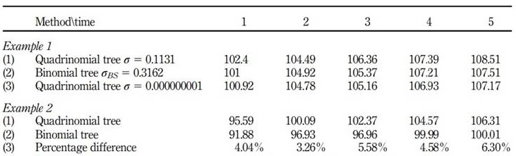
Note(s): This exhibit shows the comparison of the value of the strategic NPV through the quadrinomial method with T0 ¼ 100, K ¼ 75, V0 ¼ 0:1, α ¼ 0:01, θ ¼ 0:1, σ ¼ 0:1131 and 0:000000001, and binomial method with S0 ¼ 100 and σBS ¼ 0:3162. The table was made using MATLAB and Excel
Source(s): Own elaboration
without administrative flexibility (Brandao et al. (2012). The estimated static NPV of the project is S0 = T0 = 91:82, which was estimated according to the traditional DCF methodology using an appropriate risk-adjusted rate. The company also determined that it has an opportunity to assign the rights and property of the project to a third party at the value of K = 66 when the market conditions are unfavourable; essentially, this value corresponds to the salvage amount that remains constant over the evaluation horizon of the firms for this abandonment option. As we say above, in this case, the traditional method underestimates the strategic NPV, creating not just an erroneous valuation but violating the non-arbitrageur’s statement.
Also, the following values were obtained from a previous GARCH (1,1) estimation process of the WTI oil price yields and estimated their equivalents for the GARCH-diffusion proposed system: V0 = 0:1941, r = 0:0294, α = 0:0026, θ = 0:1941 and σ = 0:0869; and as well as: σBS = 0:3319, which was obtained using the standard deviation of the WTI returns series for the multiplicative binomial traditional methodology (see Table 4). It is worth mentioning that the estimation process is based on a quasi-maximum likelihood estimator.
Table 4 Equivalent values of the parameters for the GARCH (1,1) and GARCH-diffusion processes
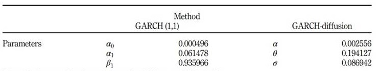
Note(s): Prepared by the authors using EViews and MATLAB
Source(s): Own elaboration
The results of the strategic NPV for periods from Year 1-5, with annual steps, are summarized in Table 5; as we can see in all the cases, the estimated values using our proposed method were higher than the traditional ones, which apparently would indicate an undervaluation of the strategic NPV by estimating lower volatility than the one presented in the yield series. Specifically, the first row shows the values for the proposed methodology; for example, for the 4th year, a strategic NPV was estimated at 104:57, with an abandonment option of 12:75, whereas, using the traditional method with multiplicative binomial trees, that is, the second row, the results corresponded to 99:99 and 8:17, respectively. The last row of Table 5 shows the percentage differences between the NPV values between the two methods, concluding that there is an approximate average 5% for all the years of the evaluation of the real options.
Table 5 Comparison of the value of the strategic NPV through the quadrinomial method and the binomial traditional method
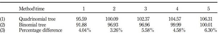
Note(s): This exhibit shows a comparison of the value of the strategic NPV using the quadrinomial method with T0 ¼ 91:82, K ¼ 66, V0 ¼ 0:1941, α ¼ 0:0026, θ ¼ 0:1941, σ ¼ 0:0869 and binomial traditional method with S0 ¼ 91:82 and σBS ¼ 0:3319. The table was made using Matlab and Excel
Source(s): Own elaboration
It is worth noting if constant volatility of 44:06% would be used in the traditional methodology, which results from finding √ θ p in the proposed method, in this case, the difference amongst the results of the two methodologies would be narrow, an element that would indicate that real option value of the traditional method would be undervalued due to a
poor estimation of the volatility in the series because such a value was greater than estimated using the standard deviation of the yields, which is commonly used.
5. Conclusions
This paper extends the literature about numerical methods for valuing derivatives, specifically for ROA valuation; the main advantage of the methodological proposed is that it includes non-constant volatility, from a formal derivation of the first two moments of a GARCH-diffusion system, to determine the probabilities of transition, growth factors and discount rates. Throughout the paper was applied a rigorous mathematical technique, which offers a relatively easy method for the public to implement and use, so it can be used to assess all types of options, in both, risk-neutral and real situations, using non-constant volatility.
The findings can be summarized as follows. First, the methodological proposed was comparable to the traditional methodology using multiplicative binomial trees as well as the closed solution proposed by Black and Scholes. The above fact occurs when the volatility in the first-mentioned method tends toward zero; since this variable is defined positive, the value of the option will vary, and this change will be in function of the values assigned to the parameters α, θ and σ that are part of the methodology proposed. Second, it was possible to use an algebraic expression to depict the evolution of the price of an asset in the presence of both dynamic and constant volatility; in this manner, its effect is captured in an appropriate way, which allows better modelling of the evolution of behaviour of the underlying asset in the market. Third, the proposed method can be used in the presence of risk neutrality through the appropriate use of a market premium, which harms the value of a call option (wait and expand) and has a positive effect on a put option (contraction and abandonment). Besides, the examples have shown that an appropriate valuation of real options is possible regardless of whether volatility is constant or not. Finally, in both examples, it was possible to verify how the inclusion of conditional and stochastic volatility in the ROA model affected the value of the real option; in the first example, it was detailed when the σ value of the proposed method changes, the strategic NPV values between the two examined methodologies differ, whereas when this variable takes values close to zero, both methodologies offer an identical solution. On another example, it was concluded that the option took a higher value in our method than the binomial method, mainly because the constant and unconditional volatility is not reflected in a time series, specifically, in the case of WTI oil commodity, the value of the option seems to be higher than its traditional simile using the multiplicative binomial method, which is explained by greater volatility obtained than estimated with standard simple yields deviation. It was also indicated, when the traditional method uses √θ p as volatility, the values of the strategic NPV were similar.
6. Discussion
Regarding the computational cost, it is possible to conclude that it is not significant since the objective of our research is to adopt the proposed numerical method to the conditions of the process itself. Strictly speaking, we want to structure a methodology with some time-series characteristics that are taken from the process, to find a more adjusted result, generating a logical discrepancy between the values of the traditional method and the proposed one. Future research aims are focus to analyse what occurs to the proposed model when there is a correlation between Wiener motions. In the other hand, it can used different commodities in real options applications to apply this proposed methodology.
In this paper, we study the particular case in which the correlation between the asset price and its volatility is zero, although many empirical studies establish that this correlation can be different from zero, as for example the model of Heston (1993).
The extension of this numerical method to models with non-zero correlation will be the subject of future work.
6.1 Practical implications
As for the practical implications, the classical methodology of real options valuation assumes that the underlying asset has constant volatility, but there is empirical and technical evidence such as that presented in Example 5.3, where it is observed that the volatility of the underlying asset is not constant and can be modelled as GARCH(1,1); not considering an adequate functional form for the volatility of any underlying asset can generate an incorrect strategic NPV estimation and consequently make unwise investment decisions. Our methodology presents reliable results, mainly because our derivation lies in a rigorous mathematical background and regarding the implementation, the multiplicative binomial recombination tends to reduce the computational cost.

