


 Inglés (pdf)
 Articulo en XML
 Referencias del artículo
 Enviar articulo por email
 Citado por SciELO
  Similares en
SciELO
Similares en
SciELO 
 Permalink
Introduction
The stability of the financial system became pertinent during the integration of the financial system and its subsequent deregulation in the 1990s (Stiglitz, 2003). The worldwide financial crisis of 2008-2009 generated great economic instability and, with it, fluctuations in the growth of the major economies, which led to a reduction in the production of imports and exports. Very few economies did not report reductions in their Gross Domestic Product (GDP) at that time. The most noticeable consequence of this financial crisis was the collapse of Lehman Brothers, the fourth-largest investment bank in the USA. This initiated the collapse of the entire American financial system (Verick and Islam, 2010). Following this event, a lot of research has been conducted to analyse the relationship between the banking system, financial stress and economic growth. Brunnermeier (2009), Adrian et al. (2010) and Davig and Hakkio (2010) conducted studies of the USA; Dhal et al. (2011) conducted studies of India; Van Roye (2011) focused on Germany and Mallick and Sousa (2013) and Apostolakis et al. (2019) analysed the impact of financial stress on European economies; however, to the best of our knowledge, this is the first study to conduct a comparative analysis of the impact of financial stress between advanced and emerging economies.
According to Smets (2014), maintaining financial stability helps ensure a well-functioning financial system, which generates efficient price stability. Likewise, macro-prudential policies can help reduce financial stress index (FSI) as they correctly manage the financial cycle, which increases the resilience of the financial sector to possible economic instability. Financial stress is a disruption in the functioning of financial markets as an incoherent intermediary between borrowers, lenders, buyers and sellers (Sandahl et al., 2011). Studying financial stress ensures that if systemic financial stress levels can be detected at an early stage, fiscal and monetary policy measures can be taken to mitigate the potential impact on the economy (Haefcket and Skarholt, 2011). Claessens and Habermeier (2013) indicate that monetary policy aims to maintain price stability. They also point out that macro-prudential policies focus on the search for financial stability. Similarly, Blot et al. (2020) argue that an unconventional monetary policy hurts sovereign yields, thus reducing the level of financial stress in the economy.
We also examined the relationship between the stock market, public debt and financial stress. Cipollini and Mikaliunaite (2020) argue that there is a transmission effect of financial stress in highly integrated markets as in the case of the Eurozone or the Latin American Integrated Market (MILA). They also posit that the level of debt has a determining effect on the transmission capacity. Jaramillo et al. (2017) argue that the level of debt affects financial markets regardless of the state of the economy, effectively reducing the returns of the stock market and increasing the yields on sovereign bonds.
We posit that this research will improve the understanding of the impact of financial stress on economic activity, as well as the channels through which financial stress increases. In addition, the index could serve as a precautionary measure against possible crises in the financial market and consequently informing measures to mitigate the impact of financial stresses on economies. This study analyses two models: the first seeks to find the relationship between GDP, inflation and financial stress in a sample of emerging and advanced economies, and the second seeks to find the relationship between the variables of the first model, the interest rate and house prices. Our hypothesis is as follows: Financial stress affects the economic growth, financial stability and monetary stability of advanced economies more than emerging economies. To prove this hypothesis, we employed panel vector autoregressive (PVAR) model techniques to investigate the correlations in financial data obtained from seven advanced economies (The USA, Canada, Germany, France, Spain, Italy and Switzerland) and seven emerging economies (Peru, Chile, Colombia, Mexico, Brazil, China and Russia) from the year 2005 to the second quarter of the year 2019. The econometric estimations show that financial stress hurts all the variables analysed more significantly in advanced economies. Our hypothesis was thus proven.
Literature review
Financial stress index
Financial stress is popularly defined as the periods in which economic agents are exposed to extreme uncertainties leading to negative expectations of financial markets (Schinasi, 2004; Allen and Wood, 2006). Illing and Liu (2006) created a financial stress index (FSI) which was applied to Canada by incorporating continuous variables where extreme values corresponded to periods of crisis. Likewise, Cardarelli et al. (2011), Balakrishnan et al. (2011) and Park and Mercado (2014) used variants of this method and applied it to emerging economies.
Van Roye (2011) constructed a financial stress measure for Germany using several bank measures, including the US Treasury Bond and the Eurodollar. Haefcket and Skarholt (2011) constructed a daily financial stress measure for Sweden by dividing the Swedish financial market into 5 parts and incorporating their individual measures into a single index, whilst Park and Mercado (2014) constructed a homogeneous measure of financial stress for 25 emerging economies.
Dhal et al. (2011) constructed a banking stability index to study the relationship between financial stability and economic growth in India. They found that economic growth, inflation and financial market stability share a medium-to-long-term relationship. They also found that financial stability can help economic growth and improve the effectiveness of monetary policies. Mallick and Sousa (2013) examined the impact of financial stress and monetary policy on the economy. They found that monetary policy shocks cause an increase in interest rate, inflation, financial stress, GDP and loan growth in the early periods following the shock. Financial stress shocks can also lead to a decrease in commodity prices, GDP, interest rates and an increase in economic growth.
Malega (2015) constructed a FSI with a specific focus on the Czech Republic, finding a significant and positive response to unemployment due to the impact of financial stress. They also found that financial stress hurts inflation and interest rates. Tng (2017) constructed a FSI for Malaysia, the Philippines and Thailand, concluding that higher-financial stress leads to tighter domestic credit conditions and lower-economic activity in all five economies, and the impact on the real economy shows a rapid initial decline followed by a gradual dissipation.
Creel et al. (2015), Stolbov and Shchepeleva (2016) and Landgren and Crook (2018) analysed the impact of financial stress on various economies, finding that financial stress hurts economic activities such as industrial production or inflation; furthermore, they highlighted the importance of macro-prudential monitoring of financial stability and the importance of central banks and policymakers in implementing tools for this purpose. Polat and Ozkan (2019) examined the impact of the financial stress in the Turkish economy; they found that the deterioration of the financial system reduces industrial production and increases inflation. They argued that stress levels should be monitored as an unconventional tool by policymakers to avoid financial instability. Ozcelebi (2020) examined the relationship between financial stresses in advanced economies with the dynamics of the exchange market in emerging economies. They concluded that high levels of financial stress can depreciate the currencies of emerging economies; this effect on the exchange rate will have a positive effect on the volatility of the stock market in the short term (Mroua and Trabelsi, 2020). Likewise, Eldomiaty et al. (2020) examine the relationship between the stock market sector, inflation and the interest rate using a cointegration model, concluding that there is a negative relationship of inflation with stock market performance, and the interest rate has a positive relationship, which is also indicating that stock market stability requires interest rate stability and robust control on inflation.
This study is related to Cardarelli et al. (2011) and Park and Mercado (2014), who employed a measure of financial stress to examine the cross-border transmission of financial stress. Balakrishnan et al. (2011) investigated how financial stress is transmitted from advanced to emerging economies. They found that the degree of financial stress is linked to the depth of financial relationships between advanced and emerging economies. Similarly, Hung (2019) conducted a study of the returns and volatility spillover of financial markets, finding that financial markets became even more integrated during the crisis, generating a volatility spillover effect that has relevant implications for policymakers. This study is also related to Apostolakis and Papadopoulos (2015) who analysed the impact of financial stress on economic growth, inflation and real estate for advanced economies in the Organisation for economic Co-operation and Development (OECD) through Panel vector autoregression (VAR). However, we extend the literature to include an analysis of the impact of financial stress in advanced and emerging economies.
Construction of the financial stress index
The construction of the FSI follows the work of Balakrishnan et al. (2011) and Park and Mercado (2014), who constructed a homogeneous FSI for advanced and emerging economies.
Banking sector
Due to the large variety of economies chosen for the sample, the heterogeneity of the sample and available data, the measure of banking stress “banking sector beta” as in Balakrishnan et al. (2011) was used. This banking sector beta follows Sharpe's (1964) Capital Asset Pricing Model (CAPM) model and is given by as follows:
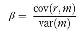
where r and m are the bank stock and market returns, respectively. The volatility of the banking sector is measured depending on the value of β; the higher the value of β, the higher the level of stress in which the banking sector is.
For the construction of the beta, we used monthly data on the average of the returns of the banks listed on each stock exchange of the economies in the sample and the return of the main stock market index of each country. The treatment of the data follows the work of Park and Mercado (2014): (1) the data were converted into year-to-year returns by taking the difference in logarithms of the current period's price with concerning last year, (2) the β was calculated using the covariance and variance of the returns in 12 months and (3) the series were transformed to take a positive value if they exceeded the value 1 and 0 otherwise.
Foreign exchange market
This study uses the conditional volatility of the monthly change in the nominal effective exchange rate quantified by a Generalized AutoRegressive Conditional Heteroskedasticity GARCH (1, 1) process. This measure is a weighted basket of the nominal exchange rate concerning the foreign currencies of a given country.
Stock market
Two stock market measures are included in the composition of the FSI. The first is stock market returns multiplied by minus one, where a decrease in returns will cause the index to increase (Apostolakis et al., 2019). The second component is stock market volatility, which is measured as a GARCH (1,1) process considering the distribution that best fits the characteristics of stock market returns. The GARCH (1,1) process proposed by Bollerslev (1986) and Engle (2001) is composed of two equations as follows:


where Equation (1) is the equation of the returns of the main stock indexes of each country, μi is the mean of r for each i and ε i is the error term for each i that follows a normal distribution N ∼ (0,1). Equation (2) specifies the conditional variance process for each hi that depends on the quadratic term of and the variance . This equation only makes sense if ω > 0, α > 0, β > 0 and α + β < 1 are satisfied (Bollerslev, 1986; Engle, 2001). This method for measuring stock market volatility and incorporating it into a stress index was used by Balakrishnan et al. (2011), Cardarelli et al. (2011) and Park and Mercado (2014). Monthly data were used, and the returns were calculated using the month-to-month difference in stock market indices.
Debt market: In this research, due to the limited availability of data on emerging economies, we chose to use the measure adopted by Cardarelli et al. (2011) research, which uses the yield spreads of the ten-year sovereign bond with respect to the US Treasury bond; in the USA, only the yield of the treasury bond will be used. This measure not only captures the systemic risk of the sovereign debt market but also any form of fiscal fragility (Rodríguez-Moreno and Peña, 2013).
Financial stress index weighting scheme
The choice of the weighting method of the financial stress components in a single index is of great importance in this construction. The method mostly used for the construction of this index is equality of variances in which the FSI is constructed by assigning each of the components similar importance and assuming that the series are normally distributed and that each series is degraded and standardised. Furthermore, equality of variances is suitable for the construction of indexes that measure the severity of financial stress in a heterogeneous sample of economies (Das et al., 2005). Each component was calculated as follows:
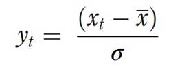
where ყt is the degraded and standardised series of each component, X is the mean of the time series and σ is the standard deviation of the series. The degraded and standardised components are then transformed into values from 0 to 1, where 1 is the largest historical value. The choice was based on the research by Cardarelli et al. (2011), Yiu et al. (2010), Park and Mercado (2014) and Apostolakis et al. (2019).
Finally, the FSI will be composed as follows:
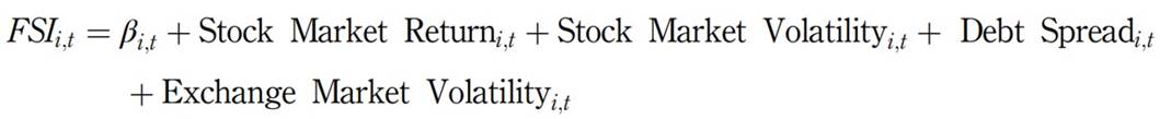
where a FSI greater than zero will mean episodes of financial stress in the economies in the sample and a value less than zero will mean that the financial markets are stable.
Methodology
Data collection
Quarterly economic growth (GDP), consumer price index (CPI), house prices (HP), short-term interest rate and FSIs' data were obtained from Bloomberg and the Bank for International Settlements (BIS). To obtain more balanced panel data and achieve consistency in findings, monthly data were converted to quarterly data. The data ranges from Q1 2005 to Q2 2019; 2019 full-year data were not considered due to unavailable data sources for both economies at the time this research took place. The sample is divided into two groups: emerging economies and advanced economies.
Table 1 shows the descriptive statistics of the sample. As can be seen, there is a higher variability of financial stress in advanced economies; furthermore, financial stress has a negative correlation with house prices and economic growth and a positive correlation with interest rate and inflation. To test the stationarity of the series, unit root tests for panel data were carried out; the tests used were Harris and Tzavalis (1999), Hadri (2000), Breitung (2005), Phillips and Perron (1988), Levin et al. (2002) and Im et al. (2003). These many tests were necessary to check for unit roots in the panel data series. The results reject the null hypothesis of the presence of unit roots in the panel data series at a 5% level of significance, except for the interest rate; therefore, this variable will be estimated in differences.
Table 1 Descriptive statistics
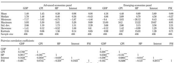
Note(s): Correlation coefficients were calculated using Pearson’s correlation test. ***, ** and * denote the level of significance at 1, 5 and 10%, respectively
Source(s): Own elaboration
Econometric estimation
We employed the PVAR model to investigate the relationship between the impact of financial stress on economic growth, and monetary and financial stability. The VAR methodology allows for the treatment of the study variables as endogenous, thus enabling us to examine the effect of the shocks of one variable on the other. Following the model of Love and Zicchino (2006), we used the PVAR model together with the generalised method of moments (GMM) to examine and compare the impact of stress between advanced and emerging economies. The PVAR model was formulated as follows:

where Yi, tis a vector of endogenous variables; Г 0 is the vector of constants; Г (L) is the matrix of polynomial lag operators; f i is the fixed effects parameter that captures time-invariant effects unobservable at the country level; d t is the forward mean difference parameter and e t is the vector of independent and identically distributed errors. The time series were disaggregated and forward skewed using the Helmert procedure as in Apostolakis et al. (2019). This was done since the fixed effects are correlated with the regressors (Arellano and Bover, 1995); likewise, the models were estimated by employing GMM-style instrumental variables as proposed by Holtz-Eakin et al. (1988).
In the following section, first, the results of the simple model and the extended five-variable model are presented; second, the Granger causality tests for each equation of the PVAR model are presented; third, the impulse response functions (IRFs) are presented. For greater accuracy of the confidence intervals, 1,000 Monte Carlo (MC) iterations are used, and finally, the forecast error variance decomposition (FEVD) is analysed.
Results
In the VAR models, the variables are arranged according to the Cholesky decomposition, which assembles the variables introduced in the model from the most exogenous to the most endogenous, followed by the introduction of macro-economic variables in the system. The models proposed for both advanced and emerging economies are as follows:
Base model: GDP - CPI - FSI
Extended model: GDP - CPI - Real estate prices - Interest rate - FSI
This ordering is since the shocks originate from the real sector of the economy and the financial sector is affected by several such shocks.
Base model
Base model estimation results
Table 2 shows the results of the PVAR (1) model for emerging and advanced economies. As can be seen, the impact of financial stress on the economy is much more significant in advanced economies on the first lag. Meanwhile, the effect of the financial stress shock on price stability, which is measured as inflation, is not significant in any of the economies.
Table 2 Base model coefficients
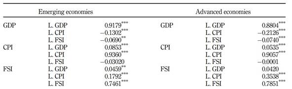
Note(s): The PVAR model was estimated with one lag according to the modified Bayesian information criterion (MBIC). No. of observations: 812 per variable; no. of panels: 14 panels. ***, ** and * denote significance level at 1 5 and 10%, respectively
Source(s): Own elaboration
Granger causality of the base model
Table 3 shows the Granger causality results of both models. The null hypothesis of this test is: FSI does not Granger-cause GDP or inflation. As can be seen, Wald statistics in the case of emerging economies indicate bidirectional causality between financial stress and economic growth, i.e. FSI has a causal effect on GDP and vice versa. In the case of advanced economies, there is unidirectional causality between FSI and GDP, and financial stress has a causal relationship with economic growth.
Table 3 Granger causality of the base model
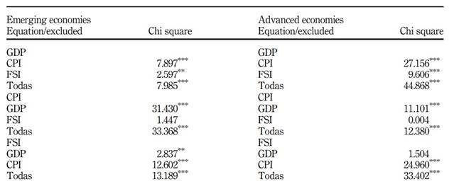
Note(s): These results are based on a three-variable PVAR model (1). Values are Wald’s chi-square statistics. ***, ** and * denote the significance level at 1, 5 and 10%, respectively
Source(s): Own elaboration
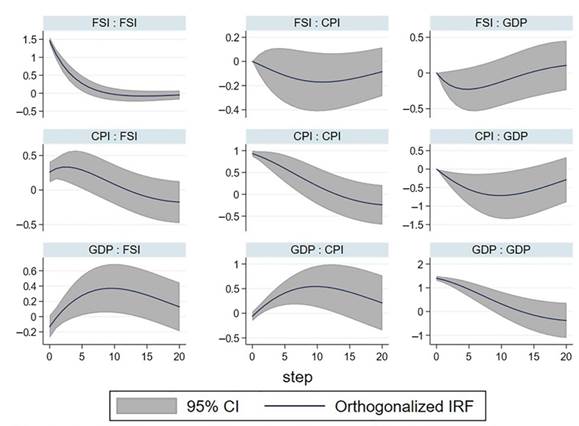
Impulse response functions
Figures 1 and 2 show the IRFs for emerging and advanced economies, respectively. They also show that in the case of emerging and advanced economies, GDP responds negatively and significantly to a financial stress shock, being more significant in the latter. These results are consistent with previous research (Mallick and Sousa, 2013; Creel et al., 2015; Apostolakis and Papadopoulus, 2015). In the case of FSI, it responds positively to shocks to CPI and economic growth in emerging economies; in the case of advanced economies, FSI responds positively to shocks to GDP and CPI. Inflation responds significantly and positively after one lag to a GDP shock in advanced and emerging economies. GDP responds negatively to CPI shocks in advanced and emerging economies. These results are also consistent with Mallik and Chowdhury (2001).
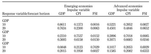
Forecast error variance decomposition (FEVD) of the base model
Table 4 shows the results of the FEVD of the PVAR base model (1), which shows that FSI in the case of advanced economies is responsible for 7% and 1.5% of the variations in GDP and CPI, respectively. For emerging economies, FSI is responsible for 1% and an average of 2% of the changes in GDP and CPI. Meanwhile, in the case of macroeconomic variables, GDP is responsible for 20% and 15% of the variations in FSI and CPI and 21% and 20% in emerging and advanced economies, respectively. Also, the results show that FSI is more responsible for GDP variations in emerging economies than advanced economies. However, in advanced economies, FSI is more responsible for CPI variations.
Extended model
Extended model estimation results
Table 5 shows the estimation results of the extended model PVAR (1); as can be seen, FSI continues to hurt GDP in both emerging and advanced economies but has only a positive and significant impact on CPI in advanced economies. Also, it can be seen that FSI hurts real estate prices in both emerging and advanced economies but only hurts interest rates in emerging economies. This finding can be attributed to European economies reducing their interest rates to negative levels from 2014 (regardless of the level of stress in their economies) as a measure for price stability.
Table 5 Extended model results for emerging and advanced economies
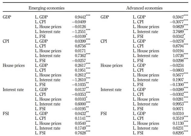
Note(s): The PVAR model was estimated with one lag according to the MBIC. No. of observations: 812 per variable; no. of panels: 14 panels. ***, ** and * denote significance level at 1, 5 and 10%, respectivel
Granger causality of the extended model
The results in Table 6 show that most variables can predict each other, i.e. they are bidirectional. In the case of emerging economies, FSI has a bidirectional relationship with house prices and a unidirectional relationship with the interest rate and the CPI; however, in advanced economies, FSI has a bidirectional relationship with the CPI and house prices and a unidirectional relationship with the interest rate.
Table 6 Granger causality of the extended model
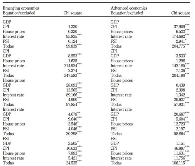
Note(s): These results are based on a 5-variable PVAR model (1). Values are Wald’s chi-square statistics. ***, ** and * denote the significance level at 1, 5 and 10%, respectively
Source(s): Own elaboration
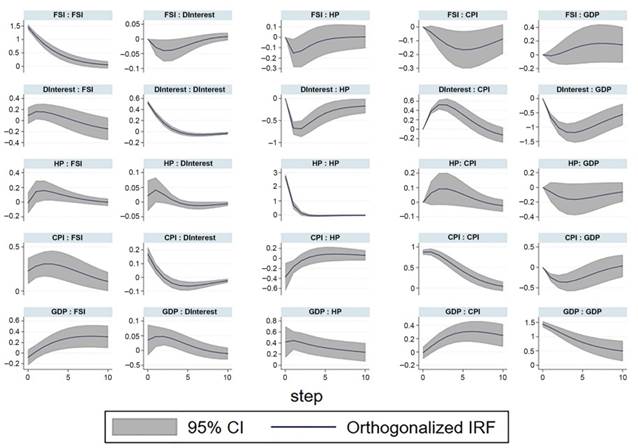
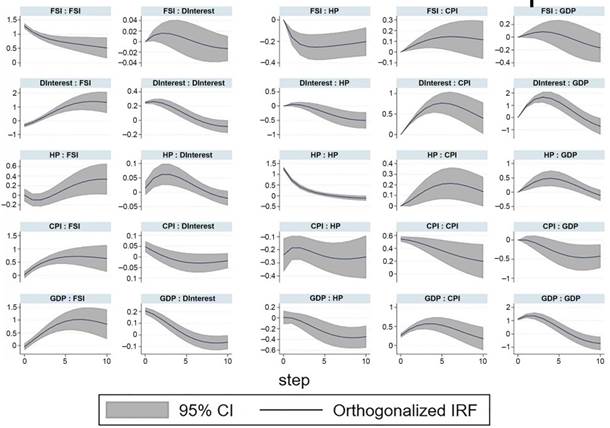
Impulse response functions of the extended model
Figures 3 and 4 show the IRFs for the emerging and advanced economies, respectively. The IRFs show that FSI shocks have similar effects on real estate prices in both emerging and advanced economies but are more significant in advanced economies. The other variables of the model do not present significant IRFs in the presence of FSI shocks. Meanwhile, the FSI is positively affected by shocks to all model variables in both emerging and advanced economies.
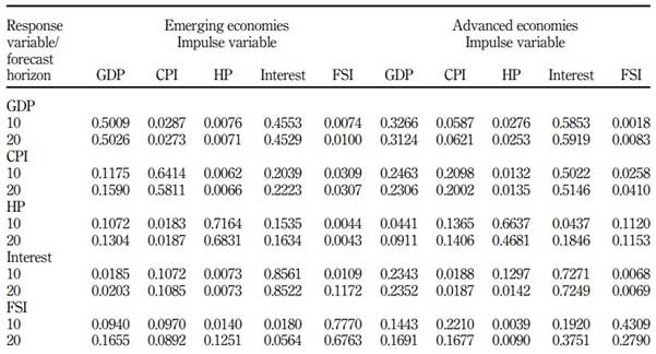
Variance decomposition (FEVD) of the extended model
Table 7 shows the results of the FEVD of the extended PVAR model (1). As can be seen, FSI and inflation are responsible for the greater proportions of the variations of GDP in emerging economies and advanced economies, respectively. Concerning the new aggregate variables, FSI is more responsible for the changes in real estate prices in advanced economies than in emerging economies, and the opposite is true for the interest rate. Meanwhile, GDP, inflation and real estate prices are more responsible for the changes in FSI in advanced economies than in emerging ones.
Discussion
Most of the results obtained in this study are consistent with previous studies. For example, Apostolakis and Papadopoulus (2015) states that financial stability should be monitored macro-prudentially through tools developed by central banks and policymakers. Our results consistently indicate a significant increase in inflation from a financial stress shock. Similarly, they also indicate that financial stress shocks hurt economic growth, government deficit and house prices. Park and Mercado (2014) state that the FSI has a great impact on economies and that a shock in the stress index can spread to other economies. Further, they posit that the financial stress of emerging economies is affected by global growth and other similar factors. Consistently, our results also show that the stress index of advanced and emerging economies affects various domestic economies; global and domestic factors also affect the stress index, and trade openness has a positive effect on financial stress. Mallick and Sousa (2013) posit that monetary policy shocks cause an increase in the interest rate, inflation, financial stress, GDP and loan growth in the first period following the shock. According to them, financial stress shocks lead to a decrease in commodity prices, GDP, interest rates and an increase in money growth. Finally, they hold that monetary policy shocks lead to an increase in the interest rate and a decrease in money growth. Similarly, our results also show that financial stress shocks lead to a decrease in economic growth and an increase in inflation.
Furthermore, Dhal et al. (2011) indicated that a bank stability index shock causes an increase in inflation and economic growth but a decrease in interest rates. In turn, an interest rate shock causes an increase in inflation and a decrease in economic growth. Consistently, in our results, the third model shows that inflation and economic growth shocks cause an increase in the interest rate. Cevik et al. (2013) constructed FSIs for five economies and examined their relationship with economic activities. Their results show that in most economies, a financial stress shock prolongs the industrial production index, as well as the other indicators of economic activity taken into consideration in their model. Further, they found that a shock of the industrial production index decreases the financial stress in that economy. Although the variables studied are not the same as in our case, they demonstrate the same impact that occurs in a scenario of a positive shock of the FSI to other exogenous variables. Finally, Kırcı Çevik et al. (2019) examined the relationship between inflation and the FSI using a Markov regime-switching model. The results show that the monetary policy of the economies analysed is consistent with the Taylor rule. They found that the low-inflation-targeting regime is more persistent and has a longer duration than the high-inflation-targeting regime. They provide evidence that financial stress has a statistically significant impact on monetary policy in the studied economies. Although they used a different model, our results are consistent with theirs.
Conclusions
We examined the differences in the impact of financial stress on economic growth, financial stability and monetary stability between advanced and emerging economies.
We found that financial stress had an impact on all the variables analysed, being more significant in advanced economies. We thus posit that financial stress affects economic growth, financial stability and monetary stability more in advanced economies.
We found a negative relationship between the stress index and economic growth, with the impact of the stress index being much greater in advanced economies. Notably, our results are consistent with most studies in the literature; however, they are more pronounced, given the methodology used for the composition of the FSI (that was calculated homogeneously for the 14 economies using the variables available in all of them.)
Inflation had a positive relationship with financial stress and a statistically significant effect on the economic activity of advanced economies. This can be attributed to the high amount of imported goods in these economies, which in high-financial stress scenarios (where the local currency depreciates) increases the local price basket.
Another important point to highlight is the relationship between the interest rate and financial stress, which shows mixed results; there is a negative relationship in the case of emerging economies, which is consistent with past research where a reduction in the interest rate occurs in scenarios of the financial crisis due to the reduction in consumption. In the case of advanced economies, we found that there is no relationship between financial stress and the interest rate. However, this can be attributed to the composition of our sample (being mostly European economies where the existing recession made them apply negative interest rate policies to reactivate the financial system regardless of the level of financial stress in the economy).
Overall, our results show that high levels of advanced economies' indebtedness to banks generate insolvency and high levels of public debt, which, in turn, increase the impact of financial stress on these economies. Meanwhile, for the emerging economies analysed, due to the low fiscal deficits that allow for greater penetration of their monetary policies to mitigate episodes of financial stress, the effect of financial stress shocks to them is diminished. Therefore, the FSI should be adapted to each economic sector and monitored by central banks to avoid liquidity problems, and monetary policy should focus on the export sector in cases of external transmission of financial stress, increasing money demand and external reserves.
Furthermore, the results obtained in this research are quite relevant for economies with high-trade openness, whose markets are exposed to the economic, financial and political problems of other economies (because financial markets are becoming increasingly integrated). Likewise, it is possible to analyse the impact of financial tensions in different economic sectors and apply appropriate measures to mitigate the impact of future economic crises.
Finally, the FSI constructed here can be incorporated as a non-conventional policy tool of economic relevance in the context of macro-prudential regulation, so central banks and policymakers can develop supervisory frameworks to examine financial stability and soundness. To reduce financial stress in their economies, central banks or monetary authorities should prioritise the stability of their banking sectors and the solvency of their financial sectors.

