


 English (pdf)
 Article in xml format
 Article references
 Send this article by e-mail
 Cited by SciELO
  Similars in
SciELO
Similars in
SciELO 
 Permalink
1. Introduction
In Mexico and other emerging economies, imports adversely influence economic growth. Thus, it is essential to correctly quantify the elasticity of import demand and the propensity to import. According to Santos-Paulino (2002 ), identifying the main variables affecting import behaviour can help policymakers design and evaluate the sustainability of an economic strategy, such as introducing an active industrial policy.
A premise in export-based growth models is that a country’s growth and development expectations improve when its exports increase and integrate into global value chains. However, as Roca and Simabuko (2015 ) mention, a paradox arises in Mexico because high export growth rates are not related to higher Gross Domestic Product (GDP) growth rates; among other reasons, they explain that it may be due to the increased propensity to import (the literature review deepens on the subject). The problem of the proportions to import, which we will study and calculate in this document, has been a topic of interest in the study of emerging economies. For example, Kovač and Kovač (2013 ) evaluate the effects of international trade in Croatia, finding that the rise in exports has been restricted by lower added value due to the growth of imports. In addition, Kaplinsky and Messner (2008 ) mention that a high level of imports could negatively affect the internal productive fabric.
This paper aims to estimate the total import demand elasticities for income, import prices and domestic prices. A high propensity to import constitutes a significant obstacle to economic growth in Mexico since the benefits of increased exports or any other aggregate demand expansion leak to the rest of the world.
This study’s main findings are that an increase of 1 peso in the Mexican GDP leads to a rise of 0.50 pesos in Mexican imports. This result has significant implications for the low impact of increased aggregate demand on GDP and economic policy (i.e. government spending to stabilize the economy). Furthermore, these findings call for a change in Mexican monetary policy regarding its economic structure to encourage an increase in the national content of its exports and domestic production.
The import demand function is estimated using a Vector Error Correction (VEC) model. After an introduction, Section 2 reviews relevant literature. Section 3 contains a brief discussion of the trends in imports, trade balance and GDP over the study period; then, we present the econometric model specification and variables. Then, Section 4 presents the results of the VEC model; and finally, Section 5 discusses the significant findings and Section 6 concludes with policy recommendations.
2. Literature review
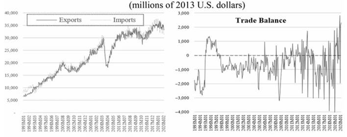
According to the recent approaches to industrial policy published by Aiginger and Rodrik (2020 ), trade policy must articulate the objectives of encouraging innovation and include a national production policy beyond seeking to correct market failures. Related to this, Guru and Yadav (2019 ) found a positive and significant relationship between financial intermediaries and economic growth in emerging economies. In the absence of financial intermediaries, Chang and Andreoni (2020 ) suggest that trade liberalization allows companies financed mainly with foreign capital to be incorporated into global value chains. This also affects internal production chains because companies with greater export activity tend to depend more on imported inputs. In addition, a weakening of the national productive structure causes the demand for consumer and investment goods to be met through imports. Andreoni (2019) explained that in an emerging economy, the positive effects of trade liberalization would only happen if the productive internal structure had a minimum level of technological capacity and human capital. According to Castillo and de Vries (2018 ), Mexico is an example of premature liberalization since productivity levels and the use of skilled workers in maquila industries have barely improved post-NAFTA. While total imports increased between 1993 and 2020 ( Figure 1 ), they do not find a systematic tendency for increased domestic sourcing of inputs. Therefore, liberalisation is not visible. This propensity to import could be an indicator to differentiate between an economy with an export vocation of added value and a maquiladora or an exporter of raw materials.
The analysis of the import demand function has become relevant in the study of emerging economies and their evolution. Therefore, there is a constant need to estimate the import demand function as new data arrives and new methods develop. Examples of this include Galindo and Cardero (1999 ), who alerts to a structural relationship between the increase of import content in Mexican exports; Zhou and Dube (2011 ) found a similar pattern for China, India, Brazil and South Africa when analyzing their import demand behaviour. Min et al. (2002 ) found for South Korea that the principal determinants of imports are the final consumption expenditure and export demand; related results had Kalyoncu (2006 ) for Turkey; Narayan and Narayan (2010 ) for South Africa; Wang and Lee (2012 ) for China; and Durmaz and Lee (2015 ) for Turkey.
Calculating the Mexican import demand is essential for its economic policy issues; since exports have expanded rapidly during the last 36 years, economic growth has stagnated. For years, many authors have blamed the industrialization pattern adopted by México as the source of low economic growth (Puyana and Romero, 2009; Moreno-Brid and Ros, 2009 ; Puyana and Romero, 2009 Romero, 2014). Since 1983, Mexican authorities have adopted an export-led growth strategy in which transnational corporations have led the export process with weak integration with the rest of the Mexican economy. This has resulted in Mexico having an extremely high import-to-export ratio ( Ruiz-Napoles, 2004 ). The exportation pattern which developed could be characterized as the “export of imports” (Romero, 2019; Ruiz-Napoles, 2020). Ibrahim (2015 ) for Saudi Arabia, Ogbonna (2016 ) for Nigeria, Muhammad and Zafar (2016 ) for Pakistan, Mishra and Mohanty (2017 ) for India and Cermeño and Rivera (2016 ) for México found in different studies a positive long-term relationship between national income or domestic consumption and the growth of imports; furthermore, all the studies report that trade balances are constantly adversely affected by higher income growth.
Since Leamer and Stern (1970 ) published their estimation of income and price elasticities of aggregate import demand, many empirical studies have been published examining the determinants of import demand and estimating import demand functions ( Khan, 1974 ; Sarmad, 1988 ; Giovannetti, 1989 ; Moran, 1989 ; Emran and Shilpi, 1996 ; Abbot and Seddighi, 1996 ; Kotan and Saygih, 1999 ; Loria, 2001 ; Lind et al., 2005 ; Ho, 2004 ; Dash, 2005 ; and Dutta and Ahmed, 2004 , among others). A general problem researchers face is choosing the form of the demand function to estimate aggregate demand models for imports. Unfortunately, international trade theory does not provide many clues about the appropriate type of specification or which equations should be used to estimate import demand. Two of the functional forms used most for this are linear and logarithmic.
3. Method
3.1 Data analysis
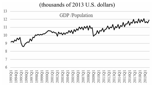
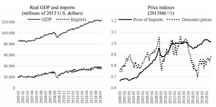
Mexico’s trade opening began 36 years ago, reaching an impressive export level equivalent to 30% of its GDP in recent years. At the same time, its imports reached the same proportion of GDP. During Mexico’s industrialization period (1940-1970), its average annual GDP growth rate was 5.99%, its per capita income 3.01% and labour productivity 2.96%. Its per capita income in 1970 was only 2.47 times greater than its 1940 GDP ( Romero, 2021 ). This high level of imports means that much of the effects of its increased exports and other components of aggregated demand leaked to the rest of the world. Figure 1 shows the evolution of the Mexican trade balance and its components since 1993. Despite the rapid increase in exports, Mexico’s GDP has grown at an annual average rate of only 2.34% annually. Its GDP per capita in 2019 was only 1.3 times greater than in 1993 (see Figure 2 ). The low impact of its exports on GDP is related to the Mexican economy’s high levels of imports. This result justifies a permanent need to estimate the import demand function for Mexico due to its essential implications for economic growth.
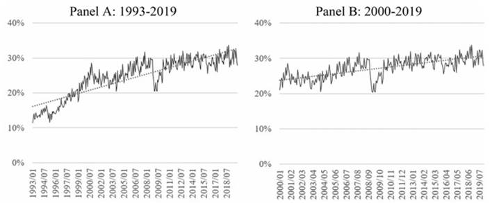
Since this data is available, estimating the import demand function for the entire 1993-2019 period is tempting. However, we would overestimate the propensity to consume given that from 1993 to 2019, the proportion of imports as a percentage of GDP went from 11.37 in January 1993 to 29.66 in January 2019. Therefore, it makes more sense to estimate the import demand function from January 2000 to December 2019 when the proportion of imports to GDP went from 21.9 in January (see Figure 3 ).
3.2 Model specification and variables
Following Leamer and Stern (1970 ), it is possible to specify the import demand equation, which relates the demanded quantity of imports to income, the price of imports and the price of domestic substitutes. The import demand equation over time t is as follows:

with Mt being the real demand of imports in foreign currency, Yf t , the national real income in foreign currency, Pm t , the price of imports and Pd t the price of domestic goods in foreign currency.
The linear formulation of aggregate import demand is expressed as follows:

α0 is the constant term in the regression, α1 is the marginal propensity to import, α2 is the coefficient of imports for foreign prices, α2 is the coefficient for domestic prices and εt is the error term.
Economic theory expects that α1 > 0, α2 < 0 and α3 > 0. However, Goldstein and Khan (1976 ) argued that if imports represent the difference between domestic consumption and production, production may grow faster or slower than consumption in response to increased real income. Therefore, imports can either increase or decrease as the actual income increases, resulting in the coefficient of α1 that is either positive or negative.
The logarithmic version of Equation (3) is written as follows:

where ln represents the natural logarithm and ut is the error term. Again, according to economic theory, it is expected that β1 >0,β2 < 0 and β3 > 0 although β1 can be negative. In previous research, for example, Khan and Ross (1977 ), Boylan et al. (1980 ) and Doroodian et al. (1994 ) have argued that the specification of the logarithmic form is preferable when import demand functions are estimated, as these forms of estimation allow the coefficients to be interpreted as elasticities of the dependent variable concerning the independent variable. This formulation mitigates the heteroscedasticity problem.
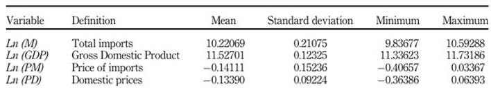
This paper uses monthly data series of total imports with their prices and the nominal exchange rate; these two series were obtained from the Bank of Mexico (System of Economic Information). The estimation uses quarterly data for real GDP in 2013 domestic prices and monthly data for the Mexican Consumer Price Index. Both series were obtained from INEGI (Bank of Economic Information), and the Two-Price Index was transformed to the 2013 base (2013M6 = 1). Real imports were obtained by dividing total nominal imports by the Price Index of Imports. To convert the real peso value of the GDP at 2013 prices, we divided the series by the nominal exchange rate of the second quarter of 2013. Also, we use the linear version of the “low to high-frequency method” to transform quarterly data into monthly data. Finally, the Consumer Price Index is divided by the normalized nominal exchange rate to obtain the Domestic Price Index (1996M6 = 1). Table 1 provides the data definitions and descriptive statistics of the studied variables.
The period used for the estimation was from January 2000 to December 2019, and total imports and the real GDP were seasonally adjusted. Figure 4 shows the variables used in the model.
3.3 Model estimation
The Augmented Dickey-Fuller test of unit root tests indicates that all series have the same level of integration I(1) ( Phillips and Hansen, 1990 ). These tests ( Table 2 ) use the four-monthly series expressed in logarithms for the 2000M01-2019M02 period (240 observations).
Table 2 Augmented Dickey Fullertest
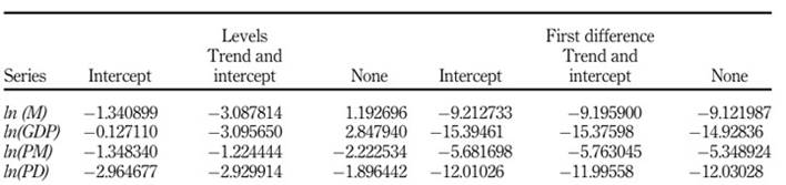
Note(s):The critical value sof the Augmented Dickey-Fuller test for intercept, trend, and intercept and none at significance levels of 1, 5 and10%are, respectively: 3.457984, 2.873596, 2.573270; 3.997418, 3.428981, 3.137946; 2.574797, 1.942176, 1.615803 Source(s):Own elaboration
As the variables are of order I(1) at 1% of significance, we estimate a Vector Auto Regression model (VAR). The VAR includes the variables ln(M), ln(GDP), ln(PM) and ln(PD). First, the correct number of lags is defined (see Table 3 ). The Criterion SC and HQ suggest two lags; AIK criteria indicate 13, LR 15 and FPE 12. To estimate the model, we used 12 lags since we worked with monthly data. A decision based on Asghar and Abid (2007) ensures the VAR system is stable and obtains a correct estimation. Additionally, they found that the FPE has a 0.85 probability of correctly estimating with 240 sample sizes. Thus, FPE is preferred over other criteria because it permits stability and correct assessment in our model.
Table 3 VAR lag order selection criteria
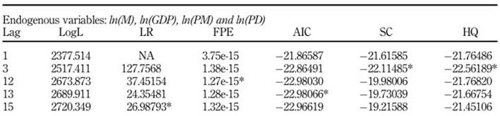
Note(s):*indicates lag order selected by the criterion LR: sequentially modified LR test statistic(each test at 5 % level); FPE: Final prediction error; AIC: Akaike informationcriterion;SC:Schwarzinformationcriterion;HQ:Hannan-Quinninformationcriterion Source(s):Own elaboration
Finally, the roots of the characteristic polynomial test show that no root lies outside the unit circle. Thus, we conclude that the VAR model satisfies the stability condition ( Pesaran and Pesaran, 1997 ).
3.4 Estimation of the VEC model
The next step for constructing the VEC model is to verify that variables are cointegrated. For that purpose, the Juselius-Johansen test performs four lags for the variables ln(M), ln(GDP), ln(PM) and ln(P.D.), and it assumes intercept (Model 3); VEC model allows for a linear deterministic trend. Included observations: 227 after adjustments. Trend assumption: Linear deterministic trend. Lags interval (in first differences): 1 to 12. The results suggest two statistics to determine the number of cointegration vectors: the trace statistic and the proof of the maximum eigenvalue (Johansen and Juselius, 1990). The critical values appropriate for the test are those given by Osterwald-Lenum (1992 ). Finally, the null hypothesis and alternative are tested using these statistics ( Table 4 ).
Table 4 Unrestricted cointegration rank test
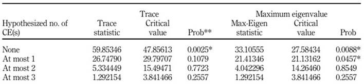
Note(s): Trace test indicates one cointegrating eqn (s) at the 0.05level *denotes rejection of the hypothesis at the 0.05 level Source(s):Own elaboration
The hypothesis of a no-cointegration can be rejected at least at 0.05 Prob. Thus, according to Johansen’s cointegration test, the model has a cointegration equation. The presence of at least one relation cointegration between the variables in levels justifies using a VEC model, combining the short-term properties of economic relationships with long-term data information in the form of a level provided by the Johansen test.
The next step is to estimate a VEC and then concentrate on the first equation:

where y is the dependent variable in the first equation of the VEC, variables xi,i51,...,4 appear as dependent on the other equations of the VEC, but as independent in the first equation, Di are exogenous variables for all the VEC and Zt−1 is the residual of the cointegration equation. The error-correction term, φ, is related to the deviation of the last period of the long-term equilibrium (the error). Therefore, it influences the short-term dynamics of the dependent variable (standard VEC estimation can be seen in Berasaluce and Romero, 2022 ). Thus, the coefficient φ measures the speed of adjustment to which the ln(M) variable returns to equilibrium after a change in the independent variables.
4. Results
As a result of the estimation of Equation (4), Table 5 shows the long-term relationship.
Table 5 Cointegration equation*
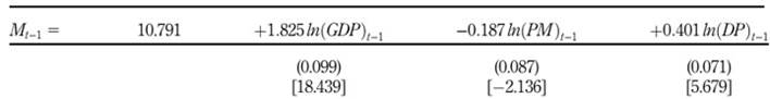
Note(s): *Standard errors in () and t-statistics in ( ).All the coefficients are significant and have the expected signs
Source(s):Own elaboration
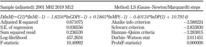
The adjusted R2 is 0.67, above 50%, so we have a good fit. We also find that the first term of error correction, φ, has the expected sign and is significant: −0.622, (0.141), (−4.398); this implies that the model returns to its equilibrium level rate of 62.2% per month. The fact that φ is less than one, statistically significant and the expected negative sign confirms a long-term joint causality of all independent variables towards imports. Also, all test results presented in Table 6 conclude that the model estimation is efficient. Furthermore, the long-term parameters of the dependent values are significant and have the expected signs according to Equation (3).
The subsequent diagnosis of the residuals consists of three parts: (a) an autocorrelation test, (b) a heteroscedasticity test and (c) a normality test.
For the Breusch-Godfrey autocorrelation test with three lags, the probability is 10.7% higher than the required 5%. Therefore, a null hypothesis is accepted, and the model has no serial correlation in the residuals at the 5% confidence level.
The Breusch-Pagan-Godfrey test analyzes heteroscedasticity in residuals; its results showed that the probability of Obs*R-squared is 65.96% higher than the 5% required. Thus, this test cannot reject the null hypothesis and concludes that the model does not hve heteroscedasticity in the residuals.
Finally, the normality test of residuals finds a value of 0.0823 for the Jarque-Bera coefficient with a probability of 0.9597. This value of 95.97% is higher than the 50% required, so the evidence cannot reject the null hypothesis, and therefore we conclude that the model presents normality in the residuals.
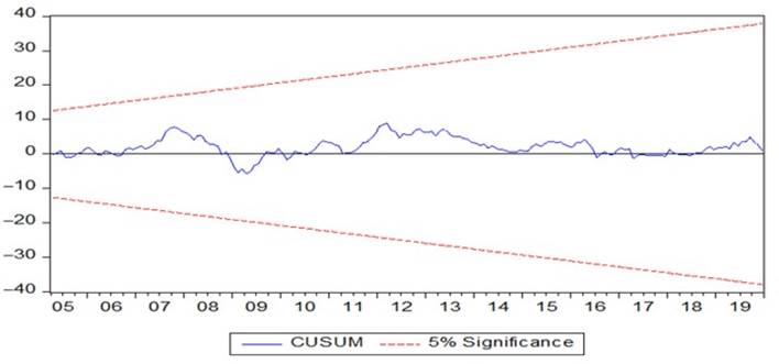
Once the model is correctly estimated, the next step is to check if the model is stable with a CUSUM test. Parameters are stable if the CUSUM line does not exceed the 5% limits (see Figure 5 ). Since these boundaries are not exceeded, the test concludes that the model is stable.
The aggregated effects of the lags of the independent variables, standard errors and t-statistics appear in Table 7 . A short-term causality exists between total imports and GDP; the cumulative effect is positive and significant. The same applies to domestic prices, which also have a positive accumulative impact on imports. In contrast, the cumulative effect of import prices on total imports is not statistically significant.
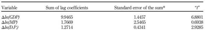
Source(s): Own elaboration
5. Discussion
5.1 Theoretical implications
Table 5 shows a high-income elasticity of import demand to GDP (1.825) and a low elasticity of import demand to import prices (0.187) and domestic prices (0.401). Although both price elasticities are low, the elasticity for domestic prices is 2.14 times greater than the elasticity for import prices. This result is a critical issue for commercial policy since low domestic prices (measured in foreign currency) help substitute imports for domestic production. An undervalued currency or increase in local productivity benefits the domestic market by reducing imports and increasing domestic demand.
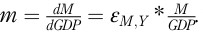
Once the aggregated import demand function is estimated, it is possible to calculate a crucial parameter for public policy: the value of the marginal propensity to import. The elasticity of import demand to income is defined as
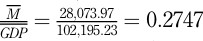
from which the marginal propensity to import is calculated as The value of εM;Y is1.825, and the estimation of using the mean value of each series is the ratio: , from which the marginal propensity to import is 0.5013 (m= 1.825 × 0.2747 = 0.5013).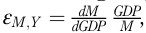

5.2 Practical implications
The high propensity to import implies that an autonomous increase in consumption, investment, government spending or exports has limited effects on national income and significant consequences for the current account balance. For example, assuming a savings propensity of 20%, the autonomous spending multiplier would
and the multiplier on the current account balance for a small-sized economy with exogenous interest rate be That is, an expansion of public spending by 1%, for example, would have an effect of 1.43% on national income and −0.71% on the current account deficit, severely reducing the effectiveness of fiscal policy as a means of stabilizing economic activity or the benefits of an expansion in exports. A country with a very open economy specializing in the labour-intensive, low-tech fragments of the global production process, such as México, develops an economic structure with high imports-to-GDP ratios and low economic growth. In general, transnational manufacturing companies move fragmented and labour-intensive production processes with low technological levels to Mexico. This is reflected in the increase in the share of imports of intermediate goods and the low relevance of imports of capital goods in total imports. In the early eighties, imports of intermediate goods accounted for 40% of total imports. By 2018, they had doubled their relative weight and reached 80% of the total. Imports of capital goods accounted for around 60% of total imports in the early eighties, but by 2018, this share had shrunk to 10%. The low weight of imports of capital goods and the large weight of imports of intermediate goods in total imports reveals the type of Mexican industrialization: a manufacturing sector that produces for both the domestic and international markets with a high content of imported intermediate goods and with little technological sophistication ( Romero, 2020 ).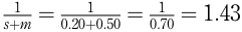

The value of the marginal propensity to import (m) is also essential to calculate the maximum GDP compatible with a zero-trade deficit
, and to compare it with the observed GDP. Also, the elasticity of imports to domestic prices (expressed in foreign currency) is 2.14 times greater than the import price elasticity; this finding could increase the local content of exports or substitute imports for local production. This last result is encouraging since an undervaluation of the currency could reduce imports and stimulate the internal market. The trade balance constraint can be relaxed to allow capital flows and resort to foreign debt, but the essence is that import requirements limit growth, directly or through increased public debt. In this sense, Dey and Tareque (2020 ) mention that many studies of developing countries report a negative relationship between external debt and economic growth.
6. Conclusions
The estimation of the aggregate demand for imports using a VEC model found that import elasticity to income is 1.825 and concluded that the propensity to import for a 1% increase in GDP is 0.5013 pesos; in other words, under current conditions, GDP growth has a significant direct effect on import demand. This high propensity to import constitutes a major obstacle to economic growth, and it limits the rate at which the economy can sustain growth without incurring significant trade deficits. Thus, emerging economies like Mexico must develop strategies that incentivize increasing aggregate domestic value on their final goods for domestic or foreign use.
The small but significant elasticity of imports to domestic prices opens the possibility for Mexico to create incentives for local producers to substitute intermediate or final goods; this can be achieved by an undervaluation of the currency or increases in productivity vis-à-vis the rest of the world. However, a more significant reduction of imports as a proportion to GDP can only be achieved through more direct policies directed at changing the structure of the Mexican economy, such as adopting active industrial policies to increase the national content of exports and the amount of goods produced locally for the domestic market.
The future research agenda should be to disaggregate the demand for imports by type of good (intermediate, final and capital goods). In addition, to better understand the effect of import demand on the Mexican economy, it would be interesting to analyze its composition by technological intensity.

