Introduction
"Quinoa can play an important role in eradicating hunger, malnutrition, and poverty", FAO Director-General said at the official launch of the "International Year of Quinoa" in February 2013. The traditional Andean crop is a so called "superfood" that has received increasing interest by consumers in high-income countries for its nutritious qualities and richness in proteins and micronutrients (Dobkin, 2008; Escuredo et al., 2014; Lester, 2006; Nowak et al., 2016). Quinoa is presented as part of the solution in the challenge of global food security, as a nutritious food for a growing world population and as an income opportunity for small-holder farmers in the Andean region (Bazile et al., 2015; Jacobsen, 2003). As a result of the increased international attention, quinoa is increasingly being traded internationally with exports from the two main producing countries, Bolivia and Peru, increasing rapidly (MINAGRI, 2018).
These international dynamics are profoundly changing the way quinoa is produced and consumed by local smallholder farmers in the Andean region. The crop is shifting from primarily being a common staple food in the region and a subsistence crop for smallholder farmers in the past (Repo-Carrasco et al., 2003) to being a high-value cash crop that is increasingly consumed in high-income countries and urban market segments (Ofstehage, 2012; Ruiz et al., 2014). Volatility and spikes in the international quinoa price create concern about the welfare of rural households in Andean regions, specifically about their quinoa consumption and the consequent implica-tions for nutrition (Macedo, 2003; Noratto et al., 2019; Vega-Gálvez et al., 2010). On the one hand, a higher quinoa price is beneficial to quinoa producers, as it increases their income. Consumers are negatively affected by a higher price and might substitute highly nutritious quinoa for other less nutritious food (Hellin and Higman, 2005; Jacobsen, 2011). Andean farm-households are at the same time consumers and producers of quinoa. Understanding the effect of a price increase on their production and consumption decisions is not straightforward, cannot be derived from theory and remains an empirical question.
In this paper, this empirical question was addressed and it was revealed whether the worldwide quinoa hype and the increased utility that high-income consumers derive from quinoa consumption comes at the expense of quinoa consumption by Andean farm-households. Specifically, the implications of changes in global quinoa prices on the production and consumption of quinoa among traditionally quinoa-producing farm-households in the Peruvian Andes were evaluated. The empirical estimation of the own price elasticity of quinoa production and consumption was underpinned with the Barnum-Squire farm-household model. This model accounts for the overall effect of farm-household behavior to changes in food prices, which simultaneously affect the consumption- and production decisions of utility maximizing farm-households (Barnum and Squire, 1979; Ellis, 1993). In its dual role as producer and consumer, the household makes interdependent production, labor allocation, and consumption decisions. The seminal Barnum-Squire farm-household model was applied using original survey data from quinoa producing households in the Junín region of the Peruvian Andes. This paper contributes a theoretically underpinned empirical investigation of the implications of changing quinoa prices for Andean farm-households, which is needed to fully understand the consequences of hyping this highly nutritious crop by international organizations and high-income consumers.
Background
Studies have analyzed the welfare implications of increasing staple food crop prices in other sectors, such as maize and rice, and have come to diverse conclusions (Dimova, 2015; Zezza et al., 2008). Some authors find a significant negative effect of higher staple food prices on food consumption (Alem and Söderbom, 2012; Attanasio et al., 2013), nutritional intake (Harttgen et al., 2016), poverty (Balagtas et al., 2014), and the mental and physical health (Hadley et al., 2012). Others find no or, among rural households, even positive effects of a price increase on staple food consumption (Hasan, 2016), self-reported food security (Verpoorten et al., 2013), and household welfare (Dimova and Gbakou, 2013) and poverty (Mghenyi et al., 2011). An older stream of literature has applied the Barnum-Squire farm-household theory to micro survey data from different countries, including Taiwan (Lau et al., 1978), Malaysia (Barnum and Squire, 1979), Korea (Ahn et al., 1981), Sierra Leone (Strauss, 1984), Mexico (Taylor and Adelman, 2002), and Bangladesh (Quayes and Rashid, 2008). These studies demonstrate that the own price elasticity of supply of staple food crops is positive but that the own price elasticity of consumption of staple food crops can be positive or negative. They conclude that the structure of the markets in which the household operates is crucial in shaping household responses to price changes. This implies that theoretically under-pinned empirical research is needed to fully understand the implications of changing quinoa prices for Andean farm-households.
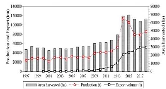
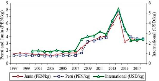
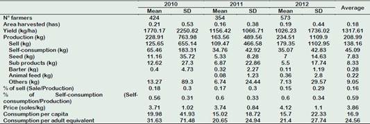
As the worldwide trade of quinoa exploded, Peru has consolidated its position as world market leader in quinoa exports, bypassing Bolivia to be the largest quinoa producer. There has been a significant increase in the harvested area, the production, and export of quinoa, with particularly sharp increases since 2012 (see Figure A in appendix). The national farm-gate quinoa price in Peru follows the international price trend very closely, and it increased considerably, from 1.16 PEN/kg on average in 1997 to 3.68 PEN/kg in 2018, corresponding to an average annual price increase of 5.7% (see Figure B in appendix). The sharpest increase is observed between 2008 and 2014 when the price jumped from 1.16 to 7.88 PEN/kg (MINAGRI, 2018). These figures clearly show that the international quinoa hype translated into a quinoa production, export, and price boom in Peru. Before 2013, quinoa was mainly a subsistence crop produced on small plots (see Table A in the appendix; Kerssen (2015)).
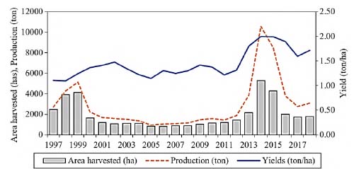
Quinoa is produced in different regions in Peru, including Andean regions where quinoa is traditionally cultivated by smallholder farmers as well as coastal regions where new large-scale production areas are being brought into cultivation. The study population was smallholder quinoa farmers in the Junín Region, which is located in the central highlands of Peru. Junín is one of the oldest quinoa-growing regions and one of the five sub-centers of genetic diversity of quinoa in Peru (Apaza et al., 2015). Within the Junín Region, seven of the nine provinces produce quinoa, but only four provinces are specialized in quinoa production: Jauja (location ratios of 6.36), Huancayo (4.96), Concepción (2.21), and Chupaca (1.10). In Junín, the area harvested and quinoa produced increased during the late 1990s but decreased sharply in 2000 and remained low until 2012, with the area fluctuating around 1000 ha and production around 1500 tons (Figure 1).
After 2012, the quinoa area and quinoa production increased sharply, with a peak of more than 5280 ha and 10551 tons in 2014, dropping slightly in 2015. Yields increased steadily during the late 1990s and early years 2000, fluctuating around 1.3 ton/ha until 2012, then increased to 1.72 tons/ha in 2018. The average quinoa farmgate price in Junín follows the same trend as the national price with an increase from 2007 onward and a peak of 7.52 PEN/kg in 2014 and a drop to 3.71 PEN/kg in 2018 (DRAJ, 2018).
Methodology and data
Barnum-Squire Model
The analysis was based on the Barnum-Squire farm-household model (Barnum and Squire, 1979; Ellis, 1993), which considers the household as an economic unit of production and consumption who trades-off the utility of consumption and the disutility of labor. In its dual role, the farm-household makes production, labor allocation and consumption decisions that are interdependent. The non-separability of production and consumption decisions can resolve an apparent paradox of positive own price elasticity of demand for food in farm-households. The household budget is endogenous and, in contrast to a pure consumer model, depends on production decisions that contribute to income through farm profits (Taylor and Adelman, 2002). The model provides an appropriate theoretical framework to analyze the response of quinoa-producing households in the Peruvian Andes to exogenous changes in quinoa prices and reflects the behavior and institutional characteristics of the Peruvian highlands.
The original Barnum-Squire model that considers four agricultural inputs (land, labor, capital and, other variable production inputs) was simplified to just three inputs (land, labor, and capital), as in Ellis (1993) and Quayes and Rashid (2008). Other specifications and assumptions remain as in the original Barnum-Squire model: the presence of a labor market and participation of farm-households in the labor market either as net buyers or net sellers of labor; no sharecropping or other contractual arrangements; a time horizon of one agricultural cycle with land availability fixed. These assumptions are consistent with the situation of farmers in the Peruvian highlands who produce quinoa both for own consumption and for the market, use both family and hired labor for production, and partly sell their labor force in the local labor market. Quinoa is grown on non-irrigated land, such that changes in the cultivated area are only possible from one agricultural season to the other.
The farm-household is assumed to maximize utility (U=𝑈(𝐿, 𝐶,𝑀, 𝑎 ?? )), a function of leisure (L), quinoa consumption (C), consumption of other (market-purchased) goods (M), and a vector of household characteristics (a i ); subject to a Cobb-Douglas quinoa pro-duction function with production (𝐹= 𝛼 0 𝐴 𝛼 1 𝐷 𝛼 2 𝐾 𝛼 3 ) a function of quinoa area (A), labor in quinoa production (D), including both household and hired labor, capital inputs (K), and a vector of parameters ( 𝛼 𝑗 ) of the jth inputs in the Cobb-Douglas production function; a time constraint (𝑇=𝐻+𝐿+𝐷); and an income constraint (𝑞𝑀+𝑝𝐶=𝑤𝐻+𝑅+𝑝𝐹− 𝑤 𝑘 𝐾).
The time constraint indicates that labor in quinoa production (D), farm-household time (L) and net labor hired in or out (H) cannot exceed the total available time of working household members (T). The income constraint indicates that the consumption of other goods bought at price q cannot exceed the income derived from quinoa production, which equals 𝑝 𝐹−𝐶 − 𝑤 𝑘 𝐾 with p quinoa price and w k capital cost; from other sources (R); and from hiring out labor at wage w, which equals wH and can be negative. It is assumed that both constraints are always binding.
In line with the original Barnun-Squire model, the household utility function was specified using the Linear Expenditure System (LES) with four arguments: C, M, L, and functions of a variety of household characteristics ( 𝑎 𝑖 ), including the number of dependents (n 2 ), the number of workers (n 1 ), and the education (e) and age (a) of the household head (eq. 1). As in the original Barnum-Squire model, farm-household time L includes leisure, reproductive and produtive work in the farm-households, apart from time allocated to quinoa production. Due to data limitations, the specification of M was modified; instead of "all other (market-purchased) goods", M refers to other food products that are consumed in lunch meals. The utility function is expressed in per capita terms to differentiate between dependents (n 2 ), allocating all time to L, and workers (n 1 ), allocating time to L and household labor in quinoa and non-farm activities (S). Dependents and workers are assumed to consume the same quantities of goods. The utility function is assumed identical and additive across individuals; can be expressed in per capita terms by dividing by n (= n 1 +n 2 ) and expressing the proportion of workers in the family with k (= n 1 /(n 1 +n 2 )) (eq. 2):
with c, m, and s being per capita consumption of quinoa (C/n), per capita consumption of other food products (M/n) and labor supply per worker (S/n 1 ); 𝛽 𝑖 parameters to be estimated for each consumption item i (C, M and L); and 𝛾 𝑖 functions of a variety of household characteristics including dependents (n 2 ), workers (n 1 ), and the education (e) and age (a) of the household head.
The time and income constraints were combined; express the equation as total household expenditures (E) on three consumption goods (C, M, and L) (eq. 3); and divide by n to obtain expression in per capita terms (eq. 4) with t-s=L/n 1 :
The farm-household constrained utility maximization problem then becomes the maximization of the utility function (eq. 2), subject to the total household expenditure constraint (eq. 4). The Lagrange function of this maximization problem is defined by:
The first-order conditions of the Lagrange maximization problem are derived in appen-dix B and result in the following set of equa-tions of household consumption of quinoa (eq. 6), consumption of other food products (eq. 7), and allocation of labor (eq. 8):
From the households' farm good demand function (eq. 6-8) and the total household expenditure function (see eq. C19 in appendix B), It is possible to derive the total proportional change in any endogenous variable Y (such as C, M or S) as a response to a proportional change in an exogenous variable X (such as w, p or q). In general, these total response elasticities are given by (Eq. 9):
Specifically, the total effect of a change in quinoa price (p) on the own-consumption of quinoa (C) or the own price elasticity of quinoa consumption 𝜂 𝑝 𝐶 is given by (Eq. 10-11):
The own price elasticity of quinoa consumption consists of two opposing effects (assuming that quinoa is a normal good). The first effect (first right-hand side term in eq. 10) is the direct effect of a change in quinoa price on the consumption of quinoa, keeping farm profits constant. This encompasses a "real income" effect stemming from a change in real income with changing quinoa prices and a "substitution" effect stemming from substitution between quinoa and other food products if quinoa prices change. This direct effect will be negative as an increase in the quinoa price decreases real income and results in substitution of quinoa for other products. The second effect (second right-hand side term in eq. 10) is the indirect effect of a change in quinoa price on the consumption of quinoa, or the "farm profit" effect. The farm-household benefits from a higher quinoa price as farm profits and total household income increase. This indirect effect is the product of two elasticities: the income elasticity of consumption ( 𝜂 𝐸 𝐶 ) and the price elasticity of income or profits ( 𝜂 𝑝 𝜋 ). The indirect effect is positive as (with quinoa assumed to be a normal good) the income elasticity of consumption and the effect of an increase in quinoa price on-farm profits are both positive. Depending on the magnitude of the two opposing effects, the positive indirect "farm profit" effect may dampen or counterbalance the negative direct "real income" and "substitution" effects. The own price elasticity of consumption of quinoa ( 𝜂 𝑝 𝐶 ) ultimately remains an empirical question. In what follows, the price elasticity of consumption of quinoa was estimated empirically using survey and secondary data from Junín. As a robustness check, additionally, the price elasticities of production and labor demand and supply and elasticities concerning wages were estimated.
Data
Data from an original cross-sectional farm-household survey that was conducted between February and March 2015 was used. Too, a three-stage sampling design with purposive selection in the first stage and stratified random selection in the second and third stage was used. In the first stage, and based on statistics collected from DRAJ (2018), 61 districts where quinoa was produced in 2014 were identified and 25 specialized in quinoa cultivation were selected (with the median of the location ratios in the last 3 years more than one). The location ratios  represent the relationship between the participation of sector "i" in region "j" and the participation of the same sector in the national total and therefore, it is used as a measure of "relative or interregional specialization". The relative specialization of a region in an activity would be associated with 𝑄 𝑖𝑗 >1; and it is measure with the harvested area (HA) between quinoa and total area cultivated (Lira and Quiroga, 2009). In the second stage, based on reports and personal communication with employees from the agricultural agencies of Concepción, Chupaca, and Jauja, the largest villages in terms of population density (154 in total) was estimated, from which samples were randomly taken from 47 villages. In the third stage, 518 farm-households were randomly selected with the number of households in each village proportional to the population of quinoa producers.
Data were obtained using a quantitative structured questionnaire with the following modules: (1) household socio-demographic characteristics; (2) land ownership; (3) quinoa production and marketing; (4) other crop production and marketing; (5) livestock and animal production; (6) off-farm activities and other income; and (7) quinoa consumption. The reference period for production and consumption data is the harvest season in 2014. The primary survey information was complemented with secondary information from DRAJ (2018), including statistics for producer and retail price data at regional, province and district levels in Junín.
Descriptive Analysis
Household demographic characteristics
Household demographic characteristics are summarized in Table 1. Thirteen percent of households in the sample are female headed; the average age of the household head is 50 years; 49% of household heads have completed secondary education, 22% have completed high education (technical institute and university) and only less than 10% have not completed primary school. The average household size (n) is 3.6 members, the average number of workers ( 𝑛 1 ) 2.07, and the number of dependents ( 𝑛 2 ) 1.54 - resulting in a workers' ratio of 0.64.
The farm-household as an economic unit of production
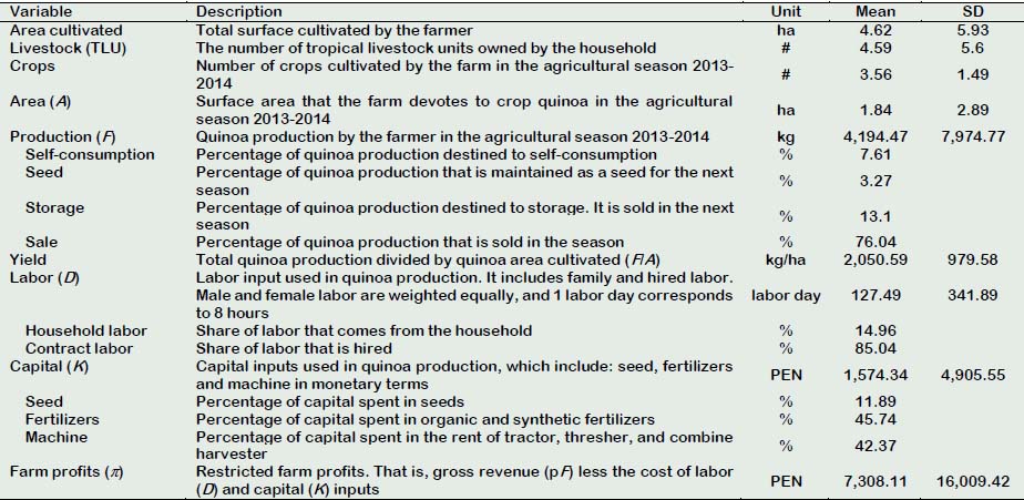
Information on the production side of the farm-household is summarized in Table 2.
Table 1 Household characteristics of quinoa producers
| Variable | Description | Unit | Mean | SD |
| Household head female | Share of female household heads | % | 12.93 | |
| Age (a) | Age of the household head | year | 50.43 | 13.43 |
| Education (e) | Education of the household head is expressed in terms of consecutive integer codes based on the level of formal education received | |||
| Primary school | Percentage of HH heads that completed primary education | % | 20.08 | |
| Secondary school | Percentage of HH heads that completed secondary education | % | 49.61 | |
| Institute | Percentage of HH heads that completed technical institute | % | 9.46 | |
| University | Percentage of HH heads that completed university | % | 12.16 | |
| Incomplete education | Percentage of HH heads with an incomplete primary education | % | 6.95 | |
| No education | Percentage of HH heads without education | % | 1.74 | |
| Family size (n) | The sum of dependents (n 2 ) and working family members (n 1 ) | # | 3.6 | 1.46 |
| Workers (n 1 ) | Members of the family that work, either on-farm or off-farm | # | 2.07 | 0.87 |
| Dependents (n 2 ) | The household members that fall in the category of student, job seeker, disabled or sick, housewife and children under the age of 8 | # | 1.54 | 1.34 |
| Proportion of workers (k) | The ratio between workers (n 1 ) and the family size (n) | # | 0.64 | 0.26 |
Note: SD, Standard deviation; HH, Household. Source: Calculations based on household survey data collected by the authors in 2015.
Table 2 Household as an economic unit of production
Note: ha, hectares. Source: Calculations based on household survey data collected by the authors in 2015.
Figures indicate that land and livestock holdings are rather small, with on average 4.62 hectares (ha) of land and 4.59 livestock units per household. The average quinoa area is 1.84 ha and the average quinoa yield 2,050.59 kg/ha. Farmers sell on average 76% of the total quinoa production in the harvest seasons, 13.1% is commercialized in the offseason, 7.61% is retained for household consumption, and 3.27% is saved as seeds for the next season. Households diversify crop production and cultivate on average 3.56 other crops, with the most common crops being potato (68% of households), corn (45%), barley (42%), broad beans (33%), wheat (19%), pea (18%), carrot (8%), and alfalfa (4%).
Farmers use on average 127.5 labor days (with one labor day equivalent to eight hours) in quinoa production, out of which 85% is hired labor and only 15% is household labor. This corroborates our assumption of an active labor market in the underlying theoretical model. The average input and capital costs (K) in quinoa production are 1,574.34 PEN, including the cost for fertilizers (45.74% of the total capital cost), machines (42.37%), and seeds (11.89%). Profits from quinoa production are on average 7,308.11 PEN, calculated as gross revenue (pF) minus the cost of labor (D) and capital (K) inputs.
The farm-household as an economic unit of consumption
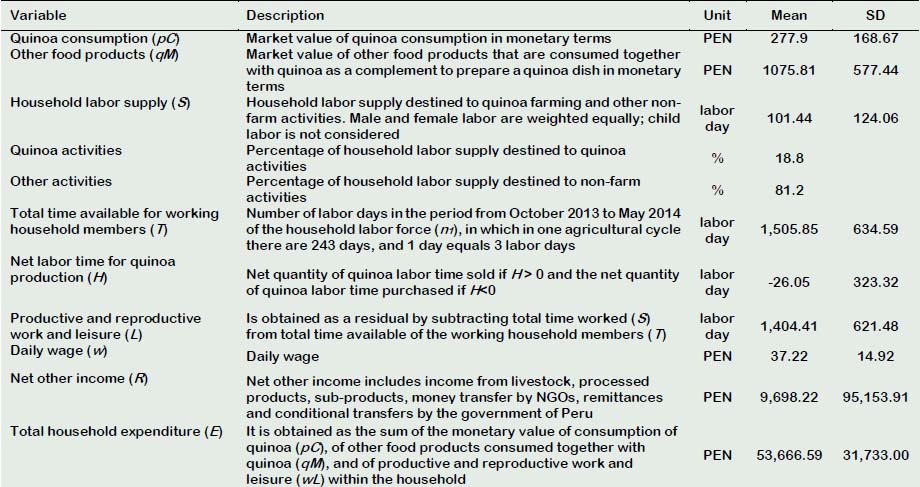
Information on the consumption of quinoa, the consumption of other food products, and the allocation of labor is summarized in Table 3. The survey data include information on the physical quantity of quinoa consumed each month for the past 12 months. The average monthly per capita quinoa consumption of households in the sample is 8.02 kg in physical terms. Due to data limitations, the consumption of quinoa and other food products is proxied for by a variable measuring the consumption of quinoa and other food products during lunch meals in the last week. As lunch is the main meal in the Peruvian Andes and as apart from small quantities at breakfast, quinoa is mainly consumed during lunch, focussing on lunch meals can proxy for the consumption of quinoa and other food products and capture the substitution of quinoa for other food products. Based on information from the survey, 104 typical lunch dishes were identified. Using information from focus group discussions with farm-households and interviews with nutritional specialists, the average amount of quinoa and other food products in these dishes was determined. This variable was multiplied with exogenous producer price data for quinoa and different food products from official district statistics (DRAJ, 2018) and add up to obtain a proxy variable for the consumption of quinoa and other food products. Prices vary across districts but not for individual producers or the districts itself. The proxy variable for quinoa (pC) and other food consumption (qM) is on average 277.90 PEN and 1,199.57 PEN respectively. The budget share of quinoa relative to other food used in an average meal is relatively small and corresponds to around 20.53% of the budget for the meal.
The total labor time available of working household members (T) in the 2014 harvest season (Oct 2013 - May 2014) is 1,506 labor days on average.
Table 3 Household as an economic unit of consumption
Note: SD, Standard deviation. Source: Calculations based on household survey data collected by the authors in 2015.
For comparability with the household reliance on hired labor, this was measured as the household labor force ( 𝑛 1 ) multiplied by the labor days in the above agricultural cycle; where the agricultural cycle corresponds to 243 days and 1 day equals 3 labor days (i.e. eight hours). The average household labor supply (S) is 101.44 labor days, where 18.80% of the labor supply is used in quinoa production and 81.20% of the household labor was destined to other non-farm activities. For the quinoa production, the households recur to hired labor (H) for an average of 26.05 labor days and at a daily wage of 37.22 PEN. This indicates that the farm-household is a buyer of quinoa-farm labor. The remaining household time (T-S) is dedicated to productive and reproductive work and leisure in the farm-household (L). It includes the activities associated with daily maintenance of the household, childcare, sleep and the production of other non-quinoa crops. The household expenditure (E) is 53,666.59 PEN and it is the sum of the monetary value of consumption of quinoa (pC), of other food products consumed together with quinoa (qM), and of productive and reproductive work and leisure (wL) within the household. The net income of any other activities of the household is 9,698.22 PEN (R); it includes income from livestock, processed products, subproducts, money transfer by NGOs, remittances and conditional transfers by the government of Peru.
Results and discussion
Survey data was used to estimate the Barnum-Squire model described in section 3, which explains the short-run production and consumption behavior of quinoa farm-households and can be used to estimate the own price elasticity of consumption of quinoa. First, the Cobb-Douglas production function is estimated by Ordinary Least Squares (OLS). From the estimated parameters the quinoa production (F), profit (𝜋), and quinoa labor demand (D) functions are obtained and the elasticities of production, profits, and labor demand concerning the price of quinoa are calculated. Second, the parameters of the expenditures equations which are nonlinear in the parameters by Feasible Generalized Nonlinear Least Squares (FGNLS) was estimated and the estimated parameters were presented for the three consumption goods. Estimated parameters were used to calculate price elasticities of consumption of quinoa (C), of consumption of other food products (M), and household labor supply in quinoa farm and non-farm activities (S). Elasticities concerning wages are estimated in both the production function and expenditure system analyses to corroborate our findings.
The Production Side
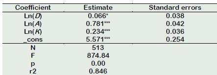
The Cobb-Douglas quinoa production function is derived (eq. 12) using the estimated production coefficients of the farm-household model that are reported in Table 4.
All coefficients are significant at the 10% level. The returns to scale are decreasing: the null hypothesis of 𝛼 1 + 𝛼 2 + 𝛼 3 =1 is rejected at the 5% significance level. The estimated coefficient for quinoa labor (D), 0.066, is relatively low. Capital (K) and area (A) are more important inputs for quinoa production, which is in line with the incre-asing mechanization of quinoa production.
Table 4 Estimates of the production side of the farm household model
Notes: * p < 0.1, ** p < 0.05, *** p < 0.01. Source: Estimations based on household survey data collected by the authors in 2015.
The quinoa production (eq. 13), profit (eq. 14), and labor demand (eq. 15) are expressed as functions of the quantity of the fixed factor (area) and the relative price of labor and capital:
These equations are used to provide estimates of the elasticities of production, labor demand, and profits of quinoa concerning price and daily wage (Table 5). The table shows that a 1% increase in quinoa price results in a 0.429% increase in quinoa production, which is small in comparison with other estimates in the literature. For Bangladesh, Quayes and Rashid (2008) estimate a production elasticity of 2.03. The smallest effect found is probably due to the approach used in this work, that is, a single agricultural good, while Quayes and Rashid (2008) consider a combination of 33 food items. Also, a 1% increase in quinoa price has a positive impact on both the demand for labor and profits, increasing both more than proportionally by 1.429%. The daily wage elasticity of quinoa production is negative. A one percent increase in the daily wage results in a 0.094% decrease in the quinoa production, and a 1.094% decline in quinoa labor demand.
The Consumption Side
The household demand function for quinoa, other food products, and household labor defined by eq. 6, 7 and 8, respectively, were estimated. Parameters with coefficients not significant at the 10% significance level were dropped and the system was reestimated. Specifically, none of the coefficients on education (e) and age of the household head (a) was found to be significant, such that, three household characteristics were used in the final estimation: household size (n), the household labor force (n 1 ), and dependents (n 2 ) (The original model by Barnum and Squire (1979) includes four variables on household characteristics: age, education, household labor force and the number of dependents). The final parameter estimates to be used for the response analysis are presented in Table 6.
Table 6 Estimated parameters of the Linear Expenditure System for an agricultural household in Junín region - Peru
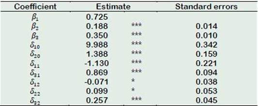
Notes: β 1 is derived from the restriction that 𝑘𝛽 1 + 𝛽 2 + 𝛽 3 =1. In calculating β 1 , k was set at its mean value of 0.637. * p < 0.1, ** p < 0.05, *** p < 0.01; N=518. Source: Estimations based on household survey data collected by the authors in 2015.
The total elasticities of household consump-tion of quinoa (C), consumption of other food products (M), and the household labor supply (S) concerning the price of quinoa (p) and the daily wage (w) are derived from the households' farm-good demand function (eq. 16) and the total household expenditure (eq. 17).
Table 7 presents the estimated elasticities, calculated at the arithmetic means of the sample. Results indicate that a one percent increase in the quinoa price (p) results in a 0.287% increase in the own-consumption of quinoa (C). This implies that the negative "real income" and "substitution" effects of increasing quinoa prices are outweighed by a positive "farm-profit" effect from quinoa production. The sign and magnitude of the estimated price elasticity of quinoa consumption of 0.287, are consistent with estimates by Lau et al. (1978) and Barnum and Squire (1979). These authors point to price elasticity of consumption of 0.221 for farm produce in Taiwan and of 0.380 for rice in Malaysia. Taylor and Adelman (2002) find a significantly larger positive price elasticity of consumption of 0.947 for staple food crops in Mexico. Other studies found significantly smaller or even negative elasticities of consumptions: Ahn et al. (1981) report an almost nil elasticity of 0.01 for rice in Korea, while both Strauss (1984) and Quayes and Rashid (2008) report respectively negative price elasticities for rice consumption in Sierra Leone (elasticity of -0.66) and a combination of crops in Bangladesh (elasticity of -0.212). Differences in findings might be related to own price elasticities and profit effects being smaller at lower expenditure levels (Strauss, 1984). Quinoa producers in Peru have higher expenditure levels than farmers in Bangladesh and Sierra Leone and are likely more similar to farmers in upper-middle-income or high-income countries like Taiwan, Malaysia or Mexico. Moreover, quinoa is a staple crop in the Peruvian Andes, but, as compared to staples in other settings is consumed in relatively small quantities, representing a comparatively small share in households' food expenditures (Vega-Gálvez et al., 2010). In this setting, income effects from increased profits through price increases are more likely to outweigh negative "real income" and "food substitution" effects.
A higher quinoa price is found to increases household labor supply, including the households' time in quinoa production and non-farm activities, by 0.651%. This likely stems from a reallocation of farm-house-hold time to on-farm quinoa production and a higher opportunity cost of farm-household time as the quinoa price increases. Moreover, it was found that a one percent increase in daily wage (w) results in an increase of own-consumption of quinoa (C) by 0.678% and a strong effect on the household labor supply (S) of 4.377%. The former two outcomes point to a positive off-farm wage-income effect while the latter reflects the higher opportunity cost of leisure due to the market wage increase.
Table 7 Household response elasticities
| Exogenous variables (X = p, w) | Total response elasticities | Own-consumption of quinoa "C" | Supply of labor "S" |
| Price of quinoa (p) | 𝜂𝑝𝑌 | 0.287 | 0.651 |
| Daily wage (w) | 𝜂Y𝑞 | 0.678 | 4.377 |
Source: Estimations based on household survey data collected by the authors in 2015.
Multicollinearity between the production factors could result in imprecise estimates of the production elasticities, which in turn could result in imprecise estimates of price elasticities. To test the robustness of the results to multicollinearity among production factors, the elasticity of own quinoa consumption concerning price was calculated using two alternative Cobb-Douglas production functions, without capital input and labor input. Very similar results as in the baseline model were found, i.e., own price elasticities of quinoa consumption of 0.282 and 0.286 respectively, pointing to the robustness of the results.
The results reveal that traditional quinoa farm-households in the central highlands of Peru increase both quinoa production and consumption as a response to an increase in the price of quinoa. In terms of the Barnum-Squire model, this implies that the positive "farm profit" effect due to the global quinoa price increase, offsets the negative "real income" and "food substitution" effects that would be predicted from the basic indifference-curve analysis. Our results do not support claims about decreasing quinoa consumption among Andean farmers (Blythman, 2013; Friedman-Rudovsky, 2012; Verner, 2013). In applying the Barnum-Squire farm-household model, the approach as similar as possible to the original model and its application by other scholars. While some applications have considered multiple farm outputs (e.g., Lau et al., 1978; Quayes and Rashid, 2008; Taylor and Adelman, 2002), the study focused on farm-households' total consumption of one staple food product, quinoa, which is in line with the original model and applications by Ahn et al. (1981) and Strauss (1984). Due to data limitations, were only considered consump-tion of quinoa and other food products in lunch meals instead of total food consumption and constructed these data based on information about the type of meals consumed in the last week. While our data do capture changes in food consumption from changes in dish composition following quinoa price increases, this is only a proxy for the consumption of non-quinoa food products or market-purchased goods. The original Barnum-Squire model and its applications, including our study, treat land as a fixed factor of production and consider only one agricultural season. Our result of positive own price elasticity of quinoa consumption, therefore, has to be interpreted as a short term effect of a changing quinoa price. In the long run and across agricultural seasons, land allocated to quinoa production and other crops may become variable and substitution of land (and labor) between crops should be taken into account, which will likely increase the "farm profit" effect and result in an even higher own price elasticity of quinoa consumption. On the other hand, increased volatility of international quinoa prices in the long run may affect farm-households' consumption and production decisions in a way that cannot be predicted by the Barnum-Squire model, which does not take into account risk behavior.
The results contribute to the literature in three ways. First, the seminal Barnum-Squire farm-household model was applied with a focus on a specific staple food crop with highly nutritious characteristics, that are not only valued in the local but also in the global market. Previous applications of the model have focused on food aggregates or staple crops with high-calorie content but the lower nutritious value and limited international market demand. Quinoa differs from common staples like rice and maize for being consumed in smaller quantities, but is, at the same time, the principal source of nutritional value for smallholder farmers in the rural Andes (Vega-Gálvez et al., 2010). Increased consumption of quinoa affects farm-households' food intake both in terms of available food quantity as well as nutritious content. Second, the emerging scientific evidence tackling the concerns about increasing quinoa prices and the consequences for smallholder quinoa producer households in Andean regions was added. Bellemare et al. (2016) point out that rising quinoa prices positively affect the total value of household consumption and household welfare. Stevens (2017) finds that cultural preferences for quinoa in certain areas of Peru do not lead to a worsening of nutritional outcomes. Our findings complement this evidence by pointing to positive own price elasticity of consumption of quinoa among traditionally quinoa-producing farm-households in the Peruvian Andes. The emerging evidence does not hold up the concerns that have arisen about the consequences of increased international demand and increasing prices for quinoa. Finally, our study is relevant in light of other global "superfoods" that are important in traditional diets in developing coun-tries but that are becoming increasingly popular for their nutritional value. Crops such as teff in Ethiopia, other Andean crops like kiwicha, kañiwa, and tarwi, coconut oil in Sri Lanka or moringa in Tanzania are traditionally cultivated for subsistence and local consumption but international demand for these crops is increasing. This can lead to important changes in consumption patterns - and consequent changes in welfare and nutrition - in areas where these crops are traditionally cultivated and understanding these effects requires empirical research.
Conclusions
The rapid increase in quinoa prices following the increased international attention to quinoa as a "superfood" and the increased international trade in quinoa, create concern about the welfare effects for (often poor) people in Andean regions, where quinoa originates from. With prices more than tripling in a couple of years, concerns have risen about Andean households' ability to further afford quinoa consumption and the consequent impact on nutrition. In this paper, the impact of the exogenous increase in the quinoa price on the own-consumption of quinoa in farm-households in the Peruvian Andes who are at the same time producers and consumers of quinoa was examined. Results show a positive impact of the increase in quinoa prices on both the production and consumption of this Andean crop in traditional quinoa-producing households. The evidence shown in this paper does not hold up the concerns that have arisen about the consequences of the quinoa hype, and the resulting increases in international demand and quinoa prices, for smallholder and poor farmers in the Andean highlands.


