


 Inglés (pdf)
 Articulo en XML
 Referencias del artículo
 Enviar articulo por email
 Citado por SciELO
  Similares en
SciELO
Similares en
SciELO 
 Permalink
Introduction
Rice (Oryza sativa L.) is the second most- produced grain in the world and plays an essential portant role in the food security for the global population (Khan et al., 2019; Asibi et al., 2019). Asian countries are responsible for over 90% of the 769 million tons of rice produced worldwide (FAOSTAT, 2018). Peru is the second most significant pro ducer in Latin America, with the highest yield rates worldwide (7.3 kg ha-1). Rice is an essential component of the basic diet of the Peruvian population, with an annual per capita consumption of 63.5 kg (Heros et al., 2014). Besides, 93% of the rice paddy in Peru is submerged and maintains flooded in most of the phenological phases; 62% of this rice cultivation is concentrated in the coastal plains (Heros et al., 2014), where irrigation is necessary to ensure productivity because the average annual rainfall is less than 90 mm (Rau et al., 2017). In such circumstances, flood irrigation remains a concern. Consequently, the current challenge is improving the water-use efficiency (WUE) to increase rice production using the least amount of water possible, reducing deep percolation, considering the low and unsteady water availability. According to Bouman and Tuong (2001), the irrigation depth applied to the rice crops can be reduced by eliminating flooding and maintaining low soil saturation conditions, thereby applying a water deficit via alternate wetting, and drying (AWD) technique. However, this AWD technique can reduce yield rates if not correctly applied and validated (Carrijo et al., 2017), particularly during the phenological stages with higher sensitivity to water stress. Crop modelling can be used to quantify the effects of water stress on crop yield (Pereira et al., 2009; Geerts et al., 2009; Shafiei et al., 2014). For rice, which might be cultivated under various water management practices, AquaCrop model was used, under drying-wetting cycles, performing well in simulating rice development, biomass and yield (Amiri, 2016; Amiri et al., 2014; Maniruzzaman et al., 2015; Xu et al., 2019a; Pirmoradian and Davatgar, 2019). Simulation models are fundamental tools to improve different management approaches in arid and semi‐arid zones for achieving maximal production with WUE (Toumi et al., 2016). The FAO AquaCrop simulation model develops in its manuals the methodology to investigate the response of crop yields (Raes et al., 2018). This model has successfully simulated the growth and yield of crops under different climate, soil, and irrigation management conditions for rice cultivation (Greaves and Wang, 2016). The AquaCrop model has been calibrated and evaluated for simulating rice development and yields under flood conditions in some areas of the world (Abdul-Ganiyu et al., 2018; Lin et al., 2012), and under drying and wetting cycles condition has been reported by Xu et al. (2019a), Amiri (2016), and Maniruzzaman et al. (2015). However, most AquaCrop studies have been based on calendar days to simulate crop development and have not been validated under irrigation management and climatic conditions of Peruvian cost. As reported by Singh et al. (2013), the application of biophysical models requires local calibration using experimental data. Consequently, the calibration of the AquaCrop model for applying the AWD technique for the coastal plains of Peru is crucial because most rice farmers use flood irrigation, with high water consumption ranging from 12000 to 20000 m3 ha-1, according to Heros et al. (2014). The present study aimed to calibrate and validate the AquaCrop model to simulate the response of rice yield to AWD irrigation under various water deficits in the central coast of Peru. The parameterization was also analyzed relative to the canopy cover development, soil water content, aerial biomass, and grain yield based on cumulative Growing Degree Days.
Materials and methods
Research area
The study was conducted in La Molina, Lima (12∘S; 76,9∘W at an altitude of 244 meters), during summer (December) 2017 and fall (April) 2018, on the central coastal plains of Peru. The climate in the coastal plains of Peru is characterized as dry, with an average monthly minimum air temperature of 12.8 °C. The average monthly maximum air temperature is 31 °C, and the average annual air temperature is 21.9 °C. The average annual precipitation is 15.5 mm.
The AquaCrop model
The AquaCrop model is based on biophysical processes (Steduto et al., 2009), considering a continuous structure of soil, plant, and atmosphere (Raes et al., 2018). The application of this model mainly includes the following four parts: Canopy cover (CC) development, biomass accumulation, SWC changes during the crop growth period, and final yield. The growth simulation models can significantly reduce the experiment duration and costs and enable better layout conditions; these attributes are suitable for the simulation of most factors and levels of the experimental plan (Zhai et al., 2019). One of the most important characteristics of the AquaCrop model is the simulation of CC. It simulates the green CC and uses reference evapotranspiration (ETo) and the crop transpiration coefficient (KcTr) values, which in turn determine the quantity of biomass produced (Singh et al., 2013; Zeleke, 2019). The AquaCrop model calculates crop transpiration (Tr) by multiplying ETo with KcTr. Tr is expressed using the following equation:
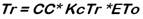 (1)
(1)
The AquaCrop model uses a standardized crop water productivity rate (WP*) to calculate the daily production of aerial biomass, which is considered constant for a climate and crop (Steduto et al., 2009; Hsiao et al., 2009).
 (2)
(2)
 (3)
(3)
In the AquaCrop model, two types of crop parameters were included: conservative and nonconservative. Conservative parameters are determined by the crop type and do not change with location, crop management method, climate, and time; therefore, predetermined values can be directly used for these parameters (Raes et al., 2009). Alternatively, nonconservative parameters are locally calibrated and validated before the model application. The model focuses on the contribution of water as the most limiting factor of the crop (Raes et al., 2009; Steduto et al., 2009). particularly in dry and semi-dry areas where water stress can vary in intensity, duration, and time of occurrence (Raoufi et al., 2018).
The AWD Irrigation Method
AWD irrigation management is a technique that has been applied to rice paddy fields and has demonstrated a reduction in the water used for irrigation. With this technique, rice paddy fields are intermittently submerged or saturated, causing upper soil layers to change from anaerobic to aerobic conditions several times during the growing season. To prevent yield reductions owing to drought stress, the field is typically resubmerged before the soil water potential (Ψw) values in the rooting area decrease to below −20 kPa (Carrijo et al., 2017; Orasen et al., 2019). Depending on the soil drying severity and duration, the farming method adopted, and local weather conditions, the number of wetting-drying cycles varies throughout the growing season. Orasen et al. (2019) reported that the AWD technique did not affect and may even increase crop yields in comparison with the flooding irrigation system. Various studies have shown that AWD could result in a 60% improvement in WUE (Carrijo et al., 2017) and up to 23% reduction in the volume of water applied via continuous flood irrigation systems (Bouman and Tuong, 2001) Although soil water condition during rice growth can affect the grain quality and associated features (Cheng et al., 2003), a recent study (Xu et al., 2019b) has reported the advantages of AWD in grain quality and nutritional value.
Experimental Treatment Procedures
A completely randomized experimental design was applied using four different AWD irrigation regimes applied under drip irrigation, with three replicates. The treatments applied were as follows:
T0. Daily irrigation, maintaining the SWC between field capacity (FC) and saturation during the growth stages of tillering (V4), primordial (V9), flowering (R4), and harvest (R9) stages (reference treatment procedure).
T1. Daily irrigation was omitted via AWD cycles, allowing the soil to dry until the threshold of SWC decrease below to −10 kPa during the V4 stage and maintaining the SWC close to saturation during the V9, R4, and R9 stages.
T2. Daily irrigation was omitted via AWD cycles, allowing the soil to dry until the threshold of SWC decrease below to −20 kPa during the V4 stage and maintaining the SWC close to saturation during the V9, R4, and R9 stages.
T3. Daily irrigation was omitted via AWD cycles, allowing the soil to dry until the threshold of SWC decrease below to −30 kPa during the V4 stage and maintaining the SWC close to saturation during the V9, R4, and R9 stages.
The experiment was conducted in 12 plots (3 × 5 m) during the summer agricultural season, with a sowing date of December 14, 2017, and a season duration of 138 days after transplantation using the IR71706 rice genotype, which exhibits high adoption po tential in Peru owing to its high production yield (Heros et al., 2014). Rice crops were cultivated via transplantation, with 20-cm spacing between rows and a density equivalent to 20000 pl ha−1. Irrigation was applied with the surface drip method, using drippers with a separation of 25 cm with a discharge of 3.7 L h−1, and an optimum fertilization dose of N, P, and K (240, 0, and 60 kg ha−1, respectively), as recommended by Heros et al. (2014).
Canopy Cover Development Measurements
CC was monitored weekly at 6 points per replicate via aerial photographs captured from above the canopy using a digital camera, as suggested by Liu and Pattey (2010). The images were analyzed using the maximum likelihood method, as described by Otukei and Blaschke (2010). In the physiological crop ripening stage, the grain yield and aerial biomass were determined for each treatment procedure following the procedures defined by Mondal et al. (2015). The biomass sample (1 m2 per plot) was obtained during the physiological ripening stage in each treatment and dried in an oven (at 70 °C) to evaluate the final biomass. The final yield was determined by harvesting 1 m2 per replicate.
Soil Water Content Measurements
SWC was measured every 30 min using a soil moisture capacitance sensor (FDR GS1, Campbell Scientific Inc., Logan, UT) placed at a depth of 20 cm in the soil in each plot used for the four treatment procedures. A frequency-domain reflectometer calibration was performed at the experimental site to measure SWC. The capacitance sensors provided proper soil moisture measurements without specific site calibration (3% - 4% precision) (Cobos et al., 2010; Leib et al., 2003). The sensors were then connected to an EM50 data recorder (Decagon Devices, Pullman, WA) to store data throughout the crop’s phenological cycle. Soil moisture was measured from December 30, 2017, to April 30, 2018. The Soil water potential (Ψw) value was obtained using the watermark granular matrix sensor (200SS, Irrometer Company, Inc., Riverside, CA) before and after each irrigation event during the AWD cycles. The readings were recorded by connecting a sensor meter that calculates soil stress within a range of 0 - 200 kPa.
AquaCrop Input
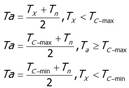
The weather input data required by the AquaCrop model, including minimum and maximum air temperatures, rainfall, wind speed, relative humidity, solar radiation, and reference crop evapotranspiration (ETo) calculated using the Penman-Monteith equation, as recommended by Allen et al. (1998), were obtained from a weather station (Davis VantagePro2, USA) located at the site of study. The data were collected during the rainy season (Decem ber 14, 2017, to April 31, 2018). The accumulated precipitation was 6,8 mm, and the average temperature was 23.44 °C. The maxi mum daily reference evapotranspiration (ETo) was calculated as 5.19 mm per day, the minimum as 1.76 mm per day, and the mean as 3.70 mm per day, is shown in Figure 1.
Growing Degree Days
For growing degree days (GDD) calculation, which is a useful index for crop growth and phenological stage (Djaman et al., 2018), the AquaCrop model used daily maximum and minimum temperatures (Raes et al., 2009) GDD were calculated using the following equations described by McMaster and Wilhelm (1997):
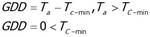 (4)
(4)
Average temperature (Ta) was estimated using the method 3 of the AquaCrop model with the following equations:
 (5)
(5)
where T c-min and T c-max are the base and upper air temperatures of the field in which the crop develops, and T x and T n are the maximum and minimum air temperatures of the day, recorded at a weather station. Although rice crop can survive under adverse temperatures between 8 °C and 30 °C (Nuruzzaman et al., 2000), for rice cultivation, the AquaCrop model considers a reference value 10 °C and 30 °C as T c-min and T c-max , respectively, for estimating GDD. However, most of the reported AquaCrop rice parameters are based on calendar days. Only Raes et al. (2018) reported a wide range of values for phenology parameters. In consequence, there is a gap in having calibrated AquaCrop parameters expressed in GDD.
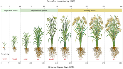
In rice cultivation, various research has been developed that describe the phenological development according to the cumulative GDD. The study employed the system proposed by Counce and Keisling (2000), which includes critical time (S0 to S3), the fully expanded leaf stages (V1 to V13), and reproductive stages (R0 to R9).
Figure 1 (a) Daily minimum and maximum air temperatures; (b) Daily rainfall and reference evapotranspiration (ETo) during the study period from December 2017 to April 2018.
These were assigned to each phenological phase based on cummulative GDD accruals for the IR71706 rice genotype, as described in Figure 2.
The IR71706 rice genotype is a highly appreciated crop to its high tolerance to water stress, with a reported yield of approximately 8 t ha−1 (Heros et al., 2014). The optimum air temperature for flowering it was between 20 °C - 27 °C.
Crop Parameters
The AquaCrop model uses three crop parameter categories: a) conservative parameters (location, cultivation, or management practices), which do not necessarily change with time, b) specific management and c) cultivation parameters, when calibrated for local conditions (Steduto et al., 2012).
Soil Data
Soil texture was characterized as sandy loam soil (15% clay, 63% sand, 22% silt). The Soil Water Characteristics Hydraulic Properties Calculator (https://hrsl.ba.ars.usda.gov/soilwater/Index.htm) was used to determine bulk density, SWC at saturation (SAT), Field capacity (FC), permanent wilting point (PMP), and saturated hydraulic conductivity, as described in Table 1.
Irrigation Data
Irrigation management comprised four irrigation regimes that maintained AWD threshold levels at Ψw = 0, −10, −15, and −20 kPa. Irrigation schedules and plans were maintained according to experimental treatments applied. Irrigation was applied using a drip irrigation system, using an automatic drip discharge of 3.75 L h-1, a pressure of 1 bar, and 95% emission uniformity. Irrigation applications were scheduled to guarantee that the level of SWC in the root zone was maintained between FC and SAT, except during the wetting-drying cycles when SWC decreased to a given AWD threshold level according to the treatments used. The amount of irrigation water applied, and the irrigation dates were monitored during the experimental periods. Because the recommended optimum fertilizer dose was applied to the study zone (Heros et al., 2014), soil fertility was not considered a limitation.
AquaCrop Model Calibration
Although the AquaCrop model recommends default growing characteristics and parameter values for rice crops, certain relevant model parameters should be locally adjusted. Basic model data was determined based on field observation data, including the meteorological data, soil data, applied irrigation, irrigation management, and initial SWC. Besides, model parameters were calibrated and validated to obtain the crop growth model applicable to the experi mental area (Zhai et al., 2019).
The model was calibrated using field information obtained from the experiment, such as CC variation and SWC, for the November 2017-April 2018 growing season.
Crop growth variables were measured, and the phenological stages were recorded. For certain parameters that were not easily measurable during the experiment, such as the KcTr, default model values were used (Raes et al., 2018). Further, nonconserva tive parameters associated with crops, soil, management, and phenological stages typi cally require an adjustment to consider local situations (Steduto et al., 2012).
During calibration, some of the most sensitive parameters of the AquaCrop model were adjusted for matching the simulation results and measured values, as reported by Geerts et al. (2008) and Salemi et al. (2011). For some of the parameters not measured during the experiment, default model values were used. Observations of phenological stages of the crop (transplantation to recovery, days to maximum CC, and days to harvest) were used in the calibration. During the process, CC and soil water content (SWC) were calibrated. Besides, final biomass was adjusted during consecutive simulations until a reasonable adjustment between the measured and simulated biomass was obtained. Other parameters were adjusted similarly.
Model Evaluation Criterion
The performance evaluation of the AquaCrop model, field measurements (observed data) were compared with CC and SWC results generated by the model (simulated data). The goodness of fit was quantified using four statistical indicators: the Nash-Sutcliffe efficiency (EF), standard deviation ratio (RSR), Willmott index (d), and determination coefficient (R2). Because each statistical indicator has its limitations, the use of a set of indicators is more robust for sufficiently assessing model performance to simulate crop growth. These indicators are shown in equations 6-9. Furthermore, Table 2 presents the performance rating based on the statistical indicator values provided by Moriasi et al. (2017) and Raes et al. (2018). Equation (6, 7, 8, 9).
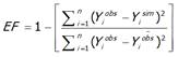 (6)
(6)
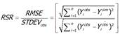 (7)
(7)
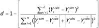 (8)
(8)
 (9)
(9)
In these equations, Y i obs and Y i sim represent the observed values and the simulated values obtained with the AquaCrop model, respectively; Y i ōbs and Y i sīm are their mean values, and n is the number of observations.
Table 2 Performance rating of statistical indicators
| Performance Rating | EF | RSR | d |
| Very good | 0.75 < EF < 1.00 | 0.00 < RSR < 0.50 | d > 0.9 |
| Good | 0.65 < EF < 0.75 | 0.50 < RSR < 0.60 | 0.80 < d < 0.89 |
| Satisfactory | 0.50 < EF < 0.65 | 0.60 < RSR ≤ 0.70 | 0.5 < d < 0.79 |
| Unsatisfactory | EF < 0.50 | RSR > 0.7 | d < 0.50 |
Source: Moriasi et al. (2017); Raes et al. (2018).
Results and discussion
Model Calibration
Calibrated parameter values are presented in Table 3. The calibration was conducted using the data collected during the November 2017-April 2018 growing season.
Table 3 Default and calibrated parameter values used in the simulation of the IR71706 rice genotype under AWD for a soil water potential of T0: −10 kPa, T1: −15 kPa, and T0: −20 kPa
| Description | Raes et al., 2018 | Used | |
| Growth and Production | |||
| Normalized water productivity WP* (g m-2) | 19 | 18.5 C | |
| Reference harvest index HI (%) | 35-50 | 43 M | |
| Phenology | |||
| Upper temperature (°C) | 30 | 30 L | |
| Base temperature (°C) | 8 | 10 L | |
| Time from transplanting to recover (GDD) | 35-100 | 50 C | |
| Time from transplanting to flowering (GDD) | 100-1300 | 1150 C | |
| Time from transplanting to start senescence (GDD) | 1000-1500 | 1300 C | |
| Time from transplanting to maturity (GDD) | 1500-2000 | 1855 C | |
| Length of the flowering state (GDD) | 300-400 | 350 C | |
| Time from Maximum effective rooting depth (GDD) | 383 | 553 C | |
| Morphology | |||
| Soil surface covered by an individual seedling at 90% recover (cm2/plant) | 3-8 | 6 C | |
| Number of plants per hectare | 300000-1500000 | 200000 C | |
| Canopy growth coefficient CGC (% GDD-1) | 6-8 | 7.9 C | |
| Maximum canopy cover CCx (%) | Almost entirely covered | 98 M | |
| Canopy decline coefficient CDC (% GDD-1) | 0.005 | 0.0046 C | |
| Maximum effective rooting depth (m) | 0.6 | 0.289 M | |
| Crop transpiration coefficient (KcTr) | 1.15 | 1.15 L | |
| Crop decrease coefficient (%/day) | 0.15 | 0.15 L | |
| Effect of canopy cover on reducing soil evaporation in late season stage (%) | 50 | 50 L | |
| Soil water depletion threshold for canopy expansion - Upper threshold | 0 | 0 L | |
| Soil water depletion threshold for canopy expansion - Lower threshold | 0.4 | 0.78 C | |
| Shape factor for Water stress coefficient for canopy expansion | 3 | 0.5 C | |
| Soil water depletion threshold for stomatal control - Upper threshold | 0.5 | 0.67 C | |
| Shape factor for Water stress coefficient for stomatal control | 3 | 0.5 C | |
| Soil water depletion threshold for canopy senescence - Upper threshold | 0.55 | 0.69 C | |
| Shape factor for Water stress coefficient for canopy senescence | 3 | 0.5 C | |
Parameters origin: Measured: M, Calibrated: C, Literature: L
Canopy Cover Development
After model calibration, the simulated values were strong correlated with the measured values. CC values under the four irrigation treatment procedures were 0.94; 0.84; 0.88; and 0.83; thereby validating the model as applicable for simulating rice crop growth.
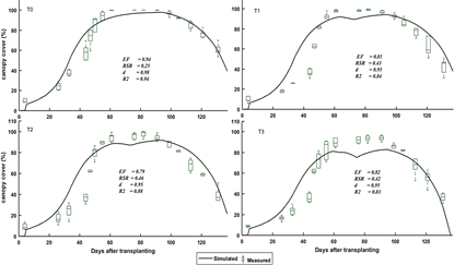
Figure 3 Canopy cover (%) measured and simulated under AWD irrigation management during the entire vegetative period of the crop, drying cycles during the vegetative tillering period, and beginning of primordial flowering (V4-V8 and R0). EF: Nash-Sutcliffe efficiency; RSR: standard deviation ratio; d: Willmott index; R2: determination coefficient.
Figure 3 presents the CC development for the entire simulated and observed crop growing season. The model showed a tendency for underestimating the CC measured during the early growing and ripening seasons, with similar results being reported by Guo et al. (2018). Also, the deficient treatment procedures (T1 and T2) exhibited CC reduction in the drying cycles during AWD irrigation, thereby miscalculating the maximum crop CC. In general, the model adequately simulated CC development (%) during the entire growing season, according to the classification provided by Moriasi et al. (2017) and Raes et al. (2018). The T0 treatment showed “very good” fitted yields at an EF of 0.94, whereas the deficit treatment procedures (T1, T2, and T3) all reported values at an EF > 80. According to Guo et al. (2018), these results indicated that model yields decrease owing to water stress.
Similarly, the model provided a high value > 0.94 and a low RSR index < 0.44 for all treatment procedures, indicating that the model can be used to simulate canopy coverage under different irrigation management re gimes. The simulated CC significantly correlated with the measured data with an R2 > 0.84. R2 values obtained were within the 0.77 - 0.98 range; this result was consistent with that reported by Amiri et al. (2016) using the AquaCrop model to simulate rice CC in Iran.
Soil Water Content
The simulation of SWC depletion during crop development is presented in Figure 4. The T0 treatment showed very good performance, with Ψw values of 0 kPa, unlike the T1, T2, and T3 treatment procedures, with Ψw values of −10, −15, and −20 kPa, respec tively; the latter treatments presented satis factory and good performances. Similar SWC depletion trends were noted between the observed and simulated data with slight overestimation tendencies. Amiri et al. (2014), Hussein et al. (2011), and Mkhabela et al. (2012) reported similar results and concluded that although the AquaCrop model properly simulated irrigation under AWD, it tended to overestimate SWC always. Similarly, statistical indicators provided high d values of > 0.79 and high EF of > 0.52 and low RSR index of < 0.7. Also, these values were significantly correlated (R2 > 0.64); therefore, the overall performance of the model was satisfactory. Besides, SWC variations between observed and simulated data may be caused by three essential fac tors: soil heterogeneity, SWC monitoring at a depth of 20 cm, unlike the AquaCrop model, which integrates SWC at a topsoil depth of 100 cm, and the contrasting water ing bulb located under each dripper.
The coefficient of determination (R2) between the measured and simulated seasonal CC was relatively high between 0.94 and 0.83, as displayed by the one to one plot (Figure 5).
The correlation for soil water content plot shown in Figure 6 indicates that the model closely simulated the grain yield with acceptable accuracy. The R2between 0.72 and 0.75 with showed a good agreement between the simulated and measured yield Overall.
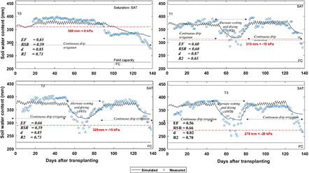
Figure 4 Soil water content (mm) measured and simulated under AWD irrigation during the entire vegetative period of the crop, drying cycles during the vegetative tillering period, and beginning of primordial flowering (V4-V8 and R0). The red dotted horizontal line indicates AWD threshold levels at treatments with soil water potential of 0, −10, −15, and -20 kPa.
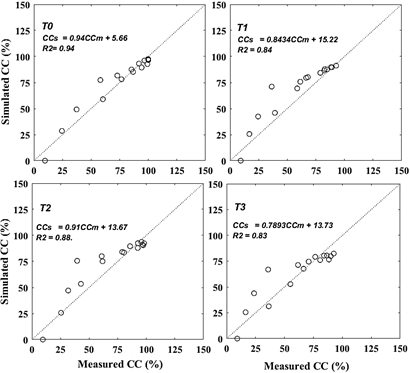
Figure 5 Correlation between measured and simulated values for soil water potential of T0: −10 kPa, T1: −15 kPa, and T0: −20 kPa for canopy cover. CCs: Canopy cover simulated; CCm: Canopy cover measured.
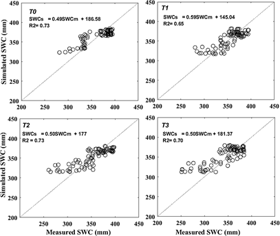
Figure 6 Correlation between measured and simulated values for soil water potential of T0: −10 kPa, T1: −15 kPa, and T0: −20 kPa for soil water content (mm).
The grain yields measured for the treat ments were 9.03; 6. 94; 5.94, and 4.68 t ha−1, which were similar to simulated results (9.05; 7.90; 5.94 and 4.68 t ha−1), with a devi ation between 0.06 and 0.84, as described in Table 4.

Water-use Efficiency
Table 5 shows the irrigation volume applied in each treatment. The volume applied for the T0 control treatment was 9189 m3 ha−1. The difference between the T0 treatment and the T3 treatment, which is the higher water deficit treatment, was 1034 m3 ha−1, representing a saving of 11%. According to Heros et al. (2014), water consumption under flood irrigation in the rice plantation areas of Peru (the Chancay-Lambayeque valleys and the upper part of the Chira-Piura valley) varies from 12000 to 20000 m3 ha−1.
Table 5 Water-use efficiency
| Treatment | Soil water potential) threshold (kPa) | Yield (kg ha−1) | Volume of water applied (m3 ha−1) | Water-use efficiency (kg/m3) |
| T0 | 0 | 10290 | 9189 | 1.12 |
| T1 | −10 | 9370 | 8781 | 1.07 |
| T2 | −15 | 6770 | 8481 | 0.80 |
| T3 | −20 | 6650 | 8155 | 0.82 |
Therefore, if compared against drip irrigation under AWD, 23% - 54% of water savings obtained. T0 and T1 treatments reduced water consumption, maintained grain yield, and improved WUE in rice, with values of 1.07 and 1.12 kg m−3, respectively. However, for the T2 and T3 treatments, WUE and yields decreased with the decrease in the volume of water applied.
The irrigation schedule optimization can effectively reduce the displacement of paddy fields and reduce the emission of paddy (Zhai et al. 2019).
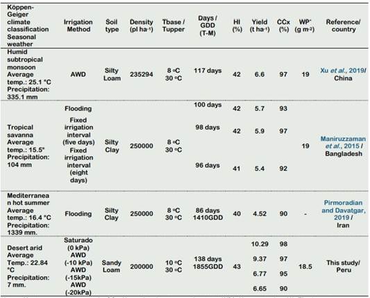
A comparison among rice AquaCrop parameters is shown in Table 6. HI was calibrated as 43%, using observed data for the unstressed treatment. CCx and WP* values were calibrated as 98 and 18.5 g m-2, respectively. Those values are similar to those reported by Xu et al. (2019a); Maniruzzaman et al. (2015); Pirmoradian and Davatgar (2019). A significant advantage of water-driven models over radiation-driven models is the opportunity to normalize the water productivity (WP*) parameter for climate, making these models widely applicable in different locations (Steduto and Albrizio, 2005; Steduto et al., 2007). For the case of measured yields, those values are higher than those cited using less plant density. However, Heros et al. (2014) reported similar yields for local varieties under flooded irrigation in Peruvian coastal-plains conditions. Results show that rice has good environmental conditions to obtain high yield with proper irrigation and agronomical management.
Table 6 Rice AquaCrop parameters reported in the literature and comparison with calibrated data in this study. The measured average values for: HI, yield, and CCx for all treatment from this study are shown
The Aquacrop model simulated the expected crop growth and the soil water content with for rice AWD conditions with reasonable performance. The FAO-recommended parameterization of the model appears to work well once the typical calibration parameters were calibrated to a local scale.
Rice Irrigation Schedule Optimization According to the AquaCrop Model
Following model calibration, an irrigation schedule was implemented under a controlled irrigation scenario to reduce irrigation depth. For these purposes, crop ETo (Table 6) was used to improve the applicability of the AquaCrop model based on controlled irrigation data collected throughout the rice growth period (December-April). The rice irrigation calendar was optimized according to rice growth data. Simulation results, considering an irrigation schedule based on crop ETo, provided the same grain yields and water savings of 36.24% compared with the T0 treatment. The T0 treatment employed daily irrigation and used a volume of 9189 m3.
Table 7 Irrigation Schedule based on AquaCrop results
| Description | Units | December | January | February | March | April | Total |
| Days in month | days | 18 | 31 | 28 | 31 | 30 | 138 |
| Net depth | mm | 8.33 | 8.33 | 8.33 | 8.33 | 8.33 | |
| Efficiency | % | 95.00 | 95.00 | 95.00 | 95.00 | 95.00 | |
| Gross depth | mm | 8.77 | 8.77 | 8.77 | 8.77 | 8.77 | |
| ETo (Penman-Monteith) | mm day−1 | 3.28 | 3.82 | 3.66 | 4.00 | 3.54 | |
| Kc (FAO) | 1.10 | 1.13 | 1.19 | 1.19 | 1.11 | ||
| Crop evapotranspiration | mm day−1 | 3.61 | 4.32 | 4.35 | 4.76 | 3.93 | |
| Irrigation frequency | day | 2 | 2 | 2 | 2 | 2 | |
| Total volume | m3 ha−1 | 650 | 1339 | 1218 | 1476 | 1179 | 5862 |
Conclusions
The results indicated that once calibrated and validated, the AquaCrop model can be used to simulate rice yields under the AWD technique, where the critical factors to be considered are the AWD threshold level and drying times applied during the phenological season.
Irrigation management strategies under AWD with Ψw values between −10 and −20 kPa during the tillering stages and at the beginning of primordial and flowering stages (V4-V8 and R0) would increase both yields and WUE. However, the threshold of Ψw below to −20 kPa would reduce yields and WUE. Therefore, if correctly implemented, the application of AWD irrigation management strategies would help improve WUE and rice availability in Peru. The framework used in the present study can be applied to validate the AquaCrop model to generate new irrigation schedules based on AWD irrigation management for rice cultivation and to develop local water management strategies. Environmental and economic impacts on WUE should be considered in further studies.

