


 Inglês (pdf)
 Artigo em XML
 Referências do artigo
 Enviar este artigo por email
 Citado por SciELO
  Similares em
SciELO
Similares em
SciELO 
 Permalink
1. Introduction
Oil palm (Elaeis guineensis L.) is one of the most widely cultivated crops in the world. Indonesia is the top producer and exporter of palm oil, with oil palm plantations covering about 12.3 million hectares. Other major producers include Colombia, Thailand, Nigeria, Papua New Guinea, and Ecuador (The World Bank, 2020). These countries account for approximately 19 million hectares or 0.39% of the world's cultivated land. The high global demand for vegetable oils and the need for alternatives to fossil fuels, such as biodiesel, are driving the expansion of agricultural frontiers into forested areas. One of the sustainable options for producing oil is using oil palm, as it is the world's most efficient oil seed crop (Gassler & Spiller, 2018; Tang & Al Qahtani, 2020).
Ecuador's oil palm crop plays a significant role in the country's agricultural sector, contributing 4.35% to the total agricultural gross domestic product (GDP) and 0.90% to the overall GDP (FAOSTAT, 2019). However, large infestations of the black palm weevil (BW) Rhynchophorus palmarum L. (Coleoptera: Curculionidae) pose a significant threat to the country's oil palm industry. A study by Guamani-Quimis et al. (2022) found that for every weevil caught in traps, oil palm net reve nue and fresh fruit bunches yield decreased by USD 343.32 per year and 0.18 tons per hectare per year, respectively, using a multiple linear regression model.
The BW is a destructive species of stem borer that primarily attacks palm trees (Arecales: Arecaceae) (Kurdi et al., 2021). The larvae of this insect feed on the terminal meristem, the tip of the crown, and fragments of the palm stem, causing the tree to rot, desiccate, and crack, potentially leading to its death (Antony et al., 2021). Originally native to certain parts of Mexico, South America, Central America, and the Caribbean, R. palmarum has become a major pest of commercial palm trees such as oil palms (E. guineensis Jacq.), coconuts (Cocos nucifera L.), and ornamental palms (Esparza-Díaz et al., 2013). In countries like Ecuador, the presence of BW may be positively correlated with the occurrence of Spear rot caused by the fungus Fusarium solani (Guamani-Quimis et al., 2022).
To ensure sustainable production of oil palm, various initiatives are being implemented to reduce negative impacts and enhance positive ones. These include the use of effective Integrated Pest Management (IPM) strategies to reduce the use of pesticides (Murguía-González et al., 2018) and the implementation of continuous monitoring systems for early detection and warning of infestations caused by pests like the weevils of the genus Rhynchophorus. These monitoring systems employ infection models based on data mining algorithms such as Naive Bayes, random forest, AdaBoost, SVM, and logistic regression (Khudri et al., 2021). To effectively detect, manage, and forecast emerging insect outbreaks, it is crucial to have a current understanding of the extent and severity of pest im pacts (Andrew, 1993). However, detecting changes in insect populations over time can be challenging (Senf et al., 2017), particularly when it comes to quantifying these changes through modeling and analysis of conditional singularities (Breiman, 2001).
The aim of analyzing a time series dataset is to develop a mathematical model that can explain the underlying process that generated it. Therefore, this study aims to investigate the use of the Autoregressive Integrated Moving Average (ARIMA) in analyzing non-stationary time series (NSTS) data of insect occurrences and its suitability for tracking insect data at a regional level. The ARIMA model combines three components, namely auto regressive, integrated, and moving average, which makes it useful for revealing both intra- and inter-annual variations in the data. It is important to note that the means, variances, and covariances of NSTS data can change over time, making it difficult to model. Thus, our study aims to contribute to the existing literature by exploring the use of ARIMA analysis for NSTS data of insect occurrences and explaining why this method is preferred over other models.
2. Materials and methods
2.1. Data collection
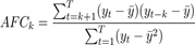
This study utilizes data collected by Guamani-Quimis et al. (2022) over a period of five growing seasons (2016-2020) from a commercial oil palm farm located (55.3 N, 79408.6 W) in Quinindé City (55.3 N, 79408.6 W), Esmeraldas Province, Ecuador. Data were collected weekly using trap counts to monitor the occurrence of BW. The distribution and classical Fourier spectrum of the data were calculated to describe the time series, with a total of 2410 observations. The data were then aggregated and treated as a monthly time series, as shown in Figure 1.
2.2. Stationary time series scale, and trend analysis
To prepare the data for modeling, we initially decomposed the time series into its seasonal, trend, and cyclical components. These innate components effectively capture the chronological information of the data and allow for better model fitting.
Y = St + Tt + Et
Y = St ∗ Tt ∗ Et(1)
where St is the seasonal component, T is the trend and cycle, and E is the remaining error.
For sequential modeling to be undertaken, the time series must be stable, with constant mean, variance, and covariance over time. To evaluate this, the Dickey-Fuller test of stationarity was used (Charemza & Syczewska, 1998; Stadnytska, 2010). The next step in selecting an ARIMA model for the time series is to determine the need for autoregression (AR) and moving average (MA) terms to accurately correct for any autocorrelation present in the differenced series. The Autocorrelation Function (ACF) plot is represented by a bar chart showing the coefficients of correlation between the time series and its lags. The Partial Autocorrelation Function (PACF) plot is represented by the partial correlation coefficient between the time series and its lags (Francq & Zakoïan, 2005). The Autocorrelation Function (ACF) was calculated using the autocorrelation equation as follows:
 (2)
(2)
where y t is the historical value in period i, y t−k is the historical value in period t-k, ӯ is the mean value, t, is the number of months, and T is the number of years in the time series. ACF and PACF were calculated using the ACPACP and APCF function of the R stats package (R Core Team, 2021).
Under the premise that y is the response variable and x 1 , x 2 , and x 3 are predictor variables in a regres sion context, PACF was determined. The correlation between the variables calculated considering how both y and x3 are related to x 1 and x 2 is known as the partial correlation between y and x 3 :
y = β 0 + β 1x2(3)
y = β 0 + β 1x + β 2x2(4)
in the first model, β 1 can be interpreted as the linear dependency between x 2 and y. In the second model, β 2 would be interpreted as the linear dependency between x 2 and y with the dependency between x and y already accounted for.
The partial autocorrelation between a time series x t and x t−h is defined as the conditional correlation between x t and x t−h , conditional on x t−h+1 , ..., x t−1 , the set of observations that come between the time points t and t − h.
2.3. ARIMA modeling
The ARIMA model was tested using different combinations of its three components p, q, and d. The parameters p and q can be expressed as:
W t = ø1 W t−1 + .... + øpW t−p + et − ø1et−1− ... − øqet−q(5)
where ø is a number between -1 and +1, p is the order of the autoregressive model, and q is the order of the moving average model. The integrated component of the model is defined in (2), with d values often set into 0, 1, or 2.
if d = 0, W t = Y t if d = 1, W t = Y t − Y t−1
if d = 2, W t = (Y t − Y t−1 ) − (Y t−1 − Y t−2 )(6)
The forecast package was used to conduct all computations (Hyndman & Khandakar, 2008). The Akaike Information Criterion (AIC) and the Bayesian Information Criterion were used to choose the components; d is the degree of differentiation and qis the order of the moving average model.) components using the Arima function (BIC). The maximal likelihood estimation (MLE) is the foundation of AIC, as illustrated in:
AIC = −2/N ∗ LL + 2k/N(7)
where N is the number of examples in the training data set, LL denotes the model's logarithmic likelihood on the training data set, and k denotes the model's parameter count. If a constant or intercept is present in the model, then k = p + q + 1; otherwise, k = p + q (Cryer, 2008). Based on the lowest AIC values discovered for various values of p, q, and d, the best values are chosen.
BIC was estimated using:
BIC = −2 ∗ LL + log (N) ∗ k(8)
where log ( ) has the base called the natural logarithm, LL is the loglikelihood of the model, N is the number of examples in the training data set, and k is the number of parameters in the model.
To facilitate finding model components (p, q, and d) we used the auto. Arima function based on Hyndman & Khandakar (2008), which returns the best ARIMA model according to either AIC or BIC value.
3. Results and discussion
Time series decomposition into seasonal, trend, and residual components using an additive decomposi tion method showed a seasonal component with a clear repeating pattern throughout the year, with negative values in the first half of the year and positive values in the second half (Figure 1). This pattern is consistent across all years, suggesting that the seasonality does not change over time. The range of the seasonal component is from -2.6333435 to 3.1492433, with the highest value in September and the lowest in February. This indicates that there is a significant seasonal effect in the data, likely due to some sort of cyclical behavior. The trend component shows an overall upward trend for most years, with the value increasing from January to December.
However, in 2020, the trend component appears to be decreasing from January to September. The range of the trend component is from 10.69562 to 16.49194, with an average growth rate of around 1.5. This indicates that there is a clear upward trend in the data, likely due to some sort of underlying growth or change. Lastly, the residual component appears to have random fluctuations without any clear pattern, indicating that the seasonal and trend components have captured most of the underlying structure in the data. The range of the residual component is from -3.73269821 to 6.95013166, with no clear pattern of behavior. This suggests that the residual component is likely due to random errors or noise in the data.
The seasonal, trend, and residual components are shown in Figure 2, which provides a visual representation of the decomposition results. Overall, the decomposition results suggest that there is a strong seasonal effect and a clear upward trend in the data, with random fluctuations accounting for the remaining variability.
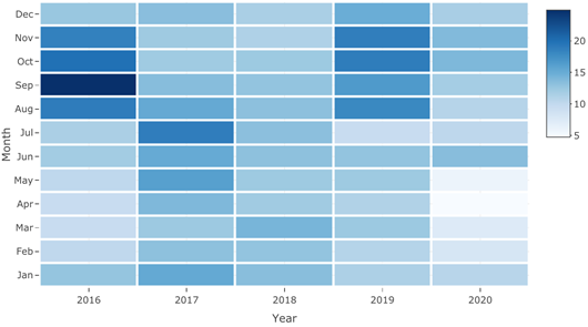
Figure 1 Heat map representation of black weevil (Rhynchophorus palmarum L.) occurrence from 2016 to 2020. The color scale indicates the level of occurrence, with darker colors representing higher levels. The heat map illustrates the temporal and seasonal variations in black weevil occurrence over the five-year period.
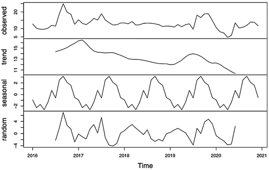
Figure 2 Decomposition of additive time series for black weevil (Rhynchophorus palmarum L.) occurrence. Panels showing the observed data (Panel A), trend component (Panel B), seasonal component (Panel C) and random component (Panel D) of the time series data. The x-axis represents the time period (years) and the y-axis represents the number of black weevil trap captures.
This indicates that ecological studies that rank R. palmarum as a high-risk pest, such as examinations of its biology, reproductive systems, and behavior during infestations, are effective tools for preventing the spread of this important agricultural pest (Camargo et al., 2010). Phenological parameters can be established in models that can be used to forecast the risks of establishment and the capacity for a growing population of R. pal marum, which include environmental, development, reproduction, and survival variables (Sporleder et al., 2013).
The results of the ACF and PACF analysis showed that there was a significant spike only at lag 1, indicating that the time series is correlated with the immediately previous observation.
Furthermore, the test showed that the variation was within the confidence interval, suggesting that it is a first-order ACF (Figure 3). The ACF by lags was used to understand the structure of the residuals of the model. The results of the ACF revealed that the series was not white noise, as there were several lags that were significantly different from zero. This pattern suggests that there may be a seasonality or trend in the time series data. A common method for modeling this pattern is by using an ARIMA (p, d, and q) model, where p represents the order of the autoregressive component, d represents the degree of differencing, and q represents the order of the moving average component. In this case, we observed high autocorrelation for the first lag (0.677) which suggests a strong relationship between the current value of the series and the lag value. The autocorrelation then decreases as the lag increases. This implies that there is no need to add AR (p) or MA (q) terms in the model. As stated by Mgaya (2019) in his study about the application of ARIMA models in forecasting livestock products consumption, the use of autocorrelation can provide valuable insights into the underlying patterns of the data and aid in the selection of an appropriate model for forecasting.
Based on the outcomes of ACF and PACF, we tried 4 distinct models prior to employing the auto-Arima algorithm (Figure 4). The bias-adjusted max imum likelihood estimator for variance (MLE) (2) for the first model (0,0,1) was 7.83, with a maximum log-likelihood (LL) of -146. The AIC and BIC were, respectively, -6.86 and -4.32. The MLE and LL for Model 2 (2,1,2) were 7.101 and 14.1, respectively, with an AIC and BIC of -8.7 and -6.3, in that order. Model 3 (3,1,1) displayed a 6.631 MLE, a -13.8 LL, and -4.82 and 2.97 AIC and BIC values. When model 4 (2,0,1) was finally evaluated, it displayed an MLE of 6.394, LL of 13.91, and AIC and BIC of 2.88 and 2.98, respectively (Figure 4). Model (2,1,2) performs best with the lowest AIC and BIC values. Other authors revealed that the effectiveness of the forecast techniques' prognostication relied heavily on the outcomes of the method for breaking down the original data and combining linear and nonlinear models via the crossing operation (Büyükşahin & Ertekin, 2019).
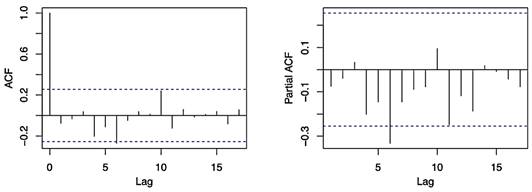
Figure 3 Auto-correlation (ACF) and partial auto-correlation (PACF) functions of the black weevil (Rhynchophorus palmarum L.) occurrence data. The x-axis represents the lag and the y-axis represents the correlation coefficient. The ACF plot shows the correlation between the black weevil occurrence data and lags of itself, and the PACF plot shows the correlation between the black weevil occurrence data and its own residuals after removing the correlation due to the lags.
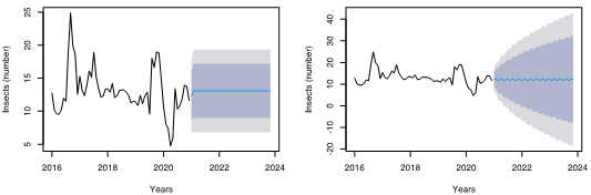
Figure 4: Fit of an Autoregressive Integrated Moving Average (ARIMA) model to univariate time series of black weevil (Rhynchophorus palmarum L.) occurrence data. The left panel shows the results of fitting a (0,0,1) model, and the right panel shows the results of fitting a (2,1,2) model. In both panels, the black line represents the original data, the blue line represents the forecasted data, and the shaded area represents the forecasted uncertainty. A forecasting was performed to forecast 48 months.
Several scientists have used ARIMA and other time series decomposition models to estimate future disease outbreaks (de Oliveira et al., 2017), crop yield (Adebiyi et al., 2014), and stock market outcome predictions (Adebayo et al., 2014). The use of auto-Arima algorithm is an important tool for identifying the best model among the different options, which is important for achieving accurate predictions. The model that we chose, the ARIMA (2,1,2), is a suitable model for forecasting the population of BW in oil palm crops.
The ARIMA (0,0,1) with non-zero mean model was fit to the BW time-series data (BWTS), resulting in coefficients of 0.5509 and 13.0781 for the moving average term and the mean, respectively, with standard errors of 0.0867 and 0.5479. The resulting model had a sigma squared value of 7.839 and a log likelihood of -146.07, leading to Akaike Information Criterion (AIC), AIC with a correction for small sample sizes (AICc), and Bayesian Information Criterion (BIC) values of 298.15, 298.58, and 304.43, respectively. This indicates that while performing prediction modeling for BW over the next two to three years, the ARIMA model's predicted outcomes are closer to the mean original historical trap data. Many academics have utilized the ARIMA model to predict the frequency and presence of pests. According to our current analysis, the BW population will decline between January and September 2021 before increasing steadily from early October 2021 to June 2023. Additionally, biological characteristics of the species, such as distinctive activity windows, flight ranges, and geographic dis tribution, might strengthen these models. However, because R. palmarum is adaptable and may easily spread far and have serious negative consequences in a range of conditions, some of these characteristics (such as geographic location) do not affect the capacity for infestation (Dalbon et al., 2021).
An ARIMA (2,1,2) model, which considers the pres ence of autoregressive terms and moving average terms of order 2, was also used to analyze BWTSD. The coefficients of the model, including the ar1 and ar2 autoregressive terms and the ma1 and ma2 moving average terms, were found to be -1.5862, -0.9977, 1.5716, and 0.9993, respectively, with standard errors of 0.0265, 0.0098, 0.0801, and 0.0927. The resulting model had a sigma squared value of 7.103 and a log likelihood of -141.15, leading to AIC, AICc, and BIC values of 292.29, 293.42, and 302.68, respectively. As observed in other studies, ARIMA models have been used to predict occurrence with significant and non-significant predictors for different pests, including Helicoverpa armigera (Noctuidae: Lepidoptera) (Narava et al., 2022), Greenhouse whitefly (Trialeurodes vaporariorum) (Chiu et al., 2019), Aphis craccivora Koch; jassids, Empoasca fabae (Harris); pod borer (Kannan et al., 2022), dengue(Lima & Laporta, 2020), rugose spiraling whitefly (Elango et al., 2020) and Black weevil (BW) in this case.
The results of the auto.arima function applied to the time series indicate that the best model found is an model (0,0,0) with a zero mean (Figure 5). This model has no autoregressive, no differencing and no moving average terms. The sigma^2 (variance of the errors) is 0.04702 and the log likelihood of the model is 6.47, which indicates a good fit of the model to the data.
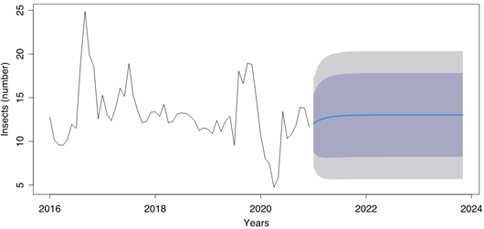
Figure 5 Time series plot of the black weevil (Rhynchophorus palmarum L.) occurrence data with the best fit ARIMA model. The x-axis represents the time period (years) and the y-axis represents the number of black weevil trap captures. The black line shows the original data, the blue line shows the forecasted data generated by the ARIMA (0,0,0) model. The shaded area represents the forecasted uncertainty.
The AIC, AICc and BIC values are -10.93, -10.86 and -8.86 respectively. These values are lower than the one from the previous models, indicating that this model is a better fit for the data. It's important to note that the time series has been differenced and logged before fitting the model, which is a common technique for making a time series stationary, and therefore, suitable for an ARIMA model.
Time series forecasting is a crucial task in various fields of science, including economics, finance, engineering, health sciences, meteorology, and agriculture. To model different social, natural, ecological, and financial phenomena, various forecasting systems have been developed. However, achieving accurate forecasting systems that can effectively model various temporal phenomena remains a significant challenge. Among the most used forecasting models are ARIMA models, which have proven to be effective due to their ability to handle non-stationary and seasonal patterns. Additionally, ARIMA models are often used as benchmark methods due to their superior performance (Montero-Manso et al., 2020).
In our study, we presented a time series model for the accurate prediction of population dynamics of the insect R. palmarum. The results of this study can be used to establish a benchmark for months with high trap captures, which can be beneficial for field pest management and decision making. While the ARIMA (0,0,0) with non-zero mean model used in this study has shown promising results. It is important to investigate the use of other types of models to forecast the BWTSD and compare their performance. Recent studies have shown that hybrid models combining ARIMA with artificial intelligence (AI) algorithms have produced superior results in predicting insect populations (Chen et al., 2023; Zhao et al., 2023). In addition, it would be worthwhile to compare the performance of ARIMA models with other time series forecasting techniques such as exponential smoothing or seasonal decomposition (Svetunkov et al., 2023). This would provide a more comprehensive understanding of the strengths and limitations of various forecasting methods for this type of time series data. Future research in this area could significantly contribute to the development of effective pest management strategies.
4. Conclusions
In our study, we investigated the use of ARIMA models for forecasting BWTSD population in a specific area. Our results indicate that the ARIMA model is a powerful tool for analyzing and forecasting time series data, particu larly data that exhibits temporal dependencies such as trends and seasonality. The analysis of the observed BWTSD revealed a consistent year-over-year pattern, with a peak in population numbers in 2017, and a decline until July 2019. By using the trained model, we were able to make forecasts for the next 24 months, providing point forecasts for each month, along with corresponding confidence intervals at the 80% and 95% levels. The forecasts were reasonable and accurately captured the underlying dynamics of the time series data. Among the four models tested, the model (0,0,0) with zero mean was found to be the best fit for the observed BWTSD. This model had no autoregressive, no differencing and no moving average terms, and had a good fit to the data as indicated by the low AIC, AICc and BIC values. Overall, our results suggest that ARIMA models can be a useful tool for forecasting time series data. They are able to capture temporal dependencies in the data and provide accurate forecasts for future periods. Future research could explore the use of ARIMA models for forecasting other types of time series data and compare their performance with other forecasting methods. Additionally, incorporating other factors such as temperature and rainfall could provide more insights into the population dynamics of R. palmarum.

