


 Inglés (pdf)
 Articulo en XML
 Referencias del artículo
 Enviar articulo por email
 Citado por SciELO
  Similares en
SciELO
Similares en
SciELO 
 Permalink
1. Introduction
It has been demonstrated that soil water content is a direct indicator of water availability for crops and can predict the impact of drought on agricultural yield better than precipitation (Xia et al., 2014). In developing countries like Peru, there is limited high-resolution spatiotemporal information about soil properties and processes, making it challenging to obtain such information for various applications (Sabino Rojas et al., 2017). Particularly, there is almost no long-term soil moisture monitoring infrastructure in developing countries (Brocca et al., 2017). Furthermore, in the context of climate change, there is an increasing need for continuous and long-term soil moisture information (Dorigo & de Jeu, 2016). In areas without instrumentation, remote sensing is a viable alternative for obtaining high-resolution and near real-time soil moisture information. Currently, the Soil Moisture Active Passive (SMAP) mission launched by NASA on January 31, 2015, is the primary dedicated remote source for continuous global soil moisture information. The soil moisture product derived from the SMAP mission, known as SMAP-L3-E (hereafter referred to as the SMAP mission), (Chan et al., 2018) provides global soil moisture information through passive observations from the radiometer aboard SMAP and offers an average accuracy of 0.05 (5%) cm3cm-3 (Das et al., 2019). However, the spatial resolution of SMAP-L3-E soil moisture estimates is approximately 9 kilometers, with an approximate temporal frequency of four days, which constitutes its main limitation (Das et al., 2019). This makes them less suitable for agricultural, hydrological, and environmental applications requiring daily and high spatial detail information (Vergopolan et al., 2021). Several methods have been proposed to enhance the spatial resolution of remote soil moisture estimates through a process called "downscaling" (Abbaszadeh et al., 2019; Bai et al., 2019; Cui et al., 2019; Fang et al., 2019; Guevara & Vargas, 2019; Hernandez-Sanchez et al., 2020; Liu et al., 2020; Mao et al., 2019; Montzka et al., 2020; Peng et al., 2017; Shangguan et al., 2024; Sishah et al., 2023; Xu et al., 2024; Zhu et al., 2023). Recently, machine learning techniques such as random forest (Hengl et al., 2018) have achieved advancements in the downscaling of remote soil moisture estimates, either spatially (Bai et al., 2019; Chen et al., 2019; Zappa et al., 2019; Zhao et al., 2018) or temporally (Lu et al., 2015; Mao et al., 2019; Xing et al., 2017). While remote sensing has proven to be a valuable tool for soil moisture measurement, in-situ observations remain essential for assessing the accuracy of soil moisture products derived from remote estimation techniques (Dorigo & de Jeu, 2016).
Our study is the first in address the problem of remote soil moisture downscaling in the Region. Furthermore, it is the only study, to the best of our knowledge, that attempts to apply a remote soil moisture downscaling approach in a context of data scarcity as commonly found in developing countries. Additionally, our study is the first of its kind to delve into the relationship between downscaled remote soil moisture and geospatial soil and terrain variables using multivariable statistical techniques (i.e., PCA).
Overall, the intention of this work is to assess a machine learning technique called random forest to enhance the spatial resolution of remote soil moisture estimates from the SMAP-L3-E product, covering the period from 2015 to 2022. Additionally, it aimed to evaluate these predictions over a hydrological year in a study area within the K´ayra watershed (Cusco, Peru).
2. Methodology
2.1 Study Area
The study area covered an approximate area of 8328 km², ranging from 72.30° W to 70.83° W and from 13.13° S to 14.68° S. This area is sufficiently large to encompass a representative number of pixels from the SMAP product with a spatial resolution of 9 km (approximately 400 pixels are covered), thus allowing for an adequate amount of satellite observations for model training.
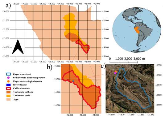
Figure 1 Location map. a) Location of the esudy region (red) within the Urubamba basin, b) shows the study region( red polygon) and location of the validation watershed (blue polygon), c) shows the validation soil moisture monitoring station (orange point) and wheter station (purple point) nearby the Kayra watershed. All plotting was done in QGIS 3.30.1-'s-Hertogenbosch.
The satellite data collection area is the Urubamba sub-basin situated within the Urubamba-Vilcanota River Basin (Figure 1). Additionally, the monitoring area is located within K´ayra micro-watershed, which is located inside the Huatanay watershed. This region experiences a dry season from May to Sept ember, coinciding with the austral winter, and a wet season from October to April, corresponding to the austral summer (Sagredo & Lowell, 2012). The mean elevation of the study area according to the SRTM3 DEM (Shuttle Radar Topography Mission 3) is 3746.95 meters, with a standard deviation of 399.48 meters.
2.2 Data Acquisition
2.2.1 The SMAP Soil Moisture Product
Launched into space in January 2015, the Soil Moisture Active Passive (SMAP) satellite, developed by the National Aeronautics and Space Administration (NASA), was designed to provide global mapping of soil moisture at high spatial and temporal resolution (Chan et al., 2018).
Soil moisture remote sensing data served as the primary component in the downscaling process. In this study, the Level 3 SMAP-L3-E product derived from the L-band radiometer on the NASA Soil Moisture Active Passive (SMAP) satellite was used. This product was obtained through NASA's Earth Observing System Data and Information System (EOSDIS).
The SMAP-L3-E product represents the average volumetric soil moisture content at a depth of approximately 5 centimeters (Entekhabi et al., 2010). The data for the SMAP product was downloaded from https://nsidc.org/data/spl3smp_e/versions/5 in GTIFF format for each available date. The data was downloaded from the start of the SMAP mission (March 31, 2015) until July of 2022 with the goal of using all available data (approximately 2000 rasters) to calibrate the proposed model.
2.2.3 Soil Properties
Geospatial information for soil physical and chemical properties at a depth of 5 cm and a spatial resolution of 250 meters was obtained for the study area using the SoilGrids system for soil property and class spatial prediction (Hengl et al., 2017) developed by ISRIC (International Soil Reference and Information Centre). The data was accessed via the following link: https://soilgrids.org/. SoilGrids offers raster-format predictions for the soil properties listed in Table 1.
Recently, Gupta et al. (2021,2022) utilized the same database and SoilGrids to derive the global distribution of soil hydraulic properties using random forest at a one-kilometer spatial resolution. These predictions were employed in the current study. An overview of the hydraulic properties used is provided in Table 2.
Additionally, the soil hydraulic properties were downloaded in GTiff format from Chue Hong (2019). The GTiff files containing soil properties were aggregated to the spatial resolution of SMAP and subsequently converted into stacks in the same manner as was done with the SMAP data.
2.2.4 Digital Elevation Model (DEM)
The digital elevation model (DEM) MERIT (Yamazaki et al., 2017) at a 90-meter spatial resolution was downloaded from http://hydro.iis.u-tokyo.ac.jp/~yamadai/MERIT_DEM/. Subsequently, the DEM was cropped and reprojected to match the study area.
Table 1 Soil properties of SoilGrids
| Soil Property⋆ | Covariate Symbol | Unit | Description |
| Organic Carbon Content | OC | g kg -1 | Gravimetric content of carbon present in soil organic matter (Nelson & Sommers, 2018). |
| Bulk Density | DA | cg cm -3 | Mass per unit volume of soil (Grossman & Reinsch, 2002). |
| Cation Exchange Capacity | CEC | cmol kg -1 | Total sum of exchangeable cations that a soil can absorb (Sumner & Miller, 2018). |
| Clay Content | Arc | g kg -1 | Gravimetric content of minerals smaller than 1 μm in size (Gee & Or, 2002). |
⋆ All variables at 250 m spatial resolution.
Table 2 Hydraulic properties of soil from Gupta et al.
| Soil properties⋆ | Covariate Symbol | Unit | Description |
|---|---|---|---|
| Saturated soil hydraulic conductivity. | KSAT | cm day -1 | Maximum water flow rate in soil under saturated conditions. |
| Saturation water content. | SVG | cm cm -3 | Volumetric water content in the soil when it reaches saturation. |
| Residual water content. | RVG | cm cm -3 | Minimum possible volumetric water content in a specific soil. |
| Parameters of the van Genuchten moisture retention function. | 𝐴𝑙𝑝ℎ𝑎, 𝑁𝑉𝐺Dimensionless | Parameters for fitting the van Genuchten function (1980). |
⋆ All variables at 1 km spatial resolution. The data can be freely accessed of Chue Hong (2019).
For processing the DEM, the terrain analysis tools of the System for Automated Geoscientific Analyses (SAGA-GIS) were employed. The processing of the DEM involved hydrological correction using the Wan and Lu method.
The topographic wetness index (TWI), also known as the topographic index or composite topographic index (Qin et al., 2007), was calculated in its original spatial resolution using equation 1:
Where A represents the drainage or catchment area (AdC), β is the local topographic slope. The concept of Topographic Wetness Index (TWI) is grounded in the principle of mass conservation, where the total catchment area is a parameter indicating the tendency to receive water, and the local slope is a parameter indicating the tendency to drain water. TWI assumes steady-state conditions and spatially invariant conditions for water infiltration and transmissivity in the soil (Gruber & Peckham, 2009)
The open-source software SAGA GIS implements various flow routing algorithms for calculating the topographic wetness index. These algorithms are summarized in Table 3.
Subsequently, the GTiff files of the DEM and topographic wetness indices were harmonized to match the spatial resolution of the SMAP product. They were then processed into stacks in the same manner as the SMAP data and soil properties.
2.2.4 PISCO Product
The PISCO product was obtained in NETCDF format from the repository of the International Research Institute for Climate and Society at Columbia University (http://iridl.ldeo.columbia.edu/). The preprocessing involved estimating historical daily precipitation averages for the four hydrological seasons, following the approach of Imfeld et al. (2021). Subsequently, the raster data were harmonized to match the spatial resolution of SMAP-L3-E. They were then processed into stacks in the same manner as the SMAP data, soil properties, and topography.
2.2.4 CHIRPS Product
Daily gridded precipitation data from the CHIRPS product (Funk et al., 2015; SENAMHI, 2015; Sun et al., 2018) were downloaded at a 5 km spatial resolution from https://climateserv.servirglobal.net/ for the period from March 2015 to July 2022 (Figure 2). Upon subsequent data analysis, it was observed that the precipitation on a specific day had limited correlation with soil moisture on the same day, at least as estimated by the SMAP product. Therefore, the arithmetic mean of the preceding 3-day precipitation was calculated and used as a covariate, omitting the precipitation for the same day.
These data underwent the same processing as the other covariates, including harmonization to match the spatial resolution of SMAP and conversion of the 2000 rasters into a single raster stack.
2.2.4 Field Soil moisture
The daily soil moisture monitoring station (orange point in Figure 1) was chosen based on accessibility and its representation of an SMAP pixel. It is located 160 meters away from the K´ayra Farm meteorological station (purple point in Figure 1) at an elevation of 3,216 meters, with the following geographic coordinates: Latitude: 13.558° S and Longitude: 71.876° W.
Soil moisture was monitored daily from May 2021 to July 2022 using the following protocol: For each measurement date, a monitoring point was located within a pixel of the downscaled SMAP product using a Garmin GPSMAP multi-band GPS device with an accuracy of approximately 1.5 meters. Once the coordinates of the sampling point were determined, three to four measurements were taken using the ThetaProbe ML3 sensor, spaced at an approximate distance of 1.5 meters from each other with the aid of a measuring tape. Subsequently, the measurements were averaged (this is permissible due to the GPS accuracy and aims to reduce soil moisture variability, as described by (Cooper, 2016). The measurements were taken at a depth of 5 cm below the soil surface (Babaeian et al., 2019). The only condition for a measurement to be considered valid is that the measured soil volume must be homogeneous and free from significant organic debris, rocks, or large cracks (NASA, 2014).
2.3 Soil moisture downscaling strategy
Our study workflow (illustrated in Figure 3) is mainly composed of 7 steps.
Table 3 Flow routing algorithms for calculating the Topographic Wetness Index (TWI), proposed in this research project
| Covariate Name | Symbol | Description | Reference |
|---|---|---|---|
| Digital Elevation Model | DEM | The algorithm divides each pixel into triangular regions, and the flow is divided towards neighboring pixels, proportional to the topographic gradient. | |
| FD8 | Fd8 | The algorithm guides the flow to all neighboring pixels with lower elevation through a flow partition exponent. | (Quinn et al., 1995) |
| MFD-md. | md | The algorithm directs the flow to all neighboring pixels with lower elevation based on the linear function of the maximum topographic gradient. | (Qin et al., 2007) |
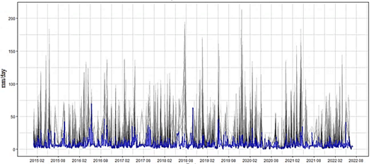
Figure 2 Daily precipitation intensity from CHIRPS product. Blue line represents the median precipitation across the entiere study region. Gray lines represent CHIRPS precipitation for all pixel inside the study reagion.

2.3.1 Step 1: Regression matrix construction
Since the original SMAP L3-- product has a 9 km resolution, all input predictors were resampled to 9 km, and stacked for each SMAP product available day. We end up having almost 2000 stacked rasters. Then, a regression matrix was constructed based on the stacks of the SMAP-L3 product and the covariates, all at the same spatial resolution. The response variable was the volumetric soil moisture content of the SMAP product for each available date. As a result, each row of the regression matrix corresponds to a specific pixel and date of the SMAP product. For static covariates, only pixel coincidence was considered. However, for dynamic covariates such as precipitation, both pixel and date coincidence with the response variable were considered. The purpose of this step was to organize the available data effectively, facilitating the development of the proposed models. Subsequently, the regression matrix was divided into two separate matrices: one for temporal disaggregation (for each pixel) and another for spatial disaggregation (for each date). These matrices were constructed using geospatial operations with the raster, sp (Pebesma & Bivand, 2005), and dplyr (Wickham et al., 2022) libraries in R.
2.3.2 Step 2: Random Forest training
In this research we propose a simple downscaling method based on the Random Forest algorithm (Hengl et al., 2018; Heung et al., 2016; Zhao et al., 2018). Random Forests (Breiman, 2001), is ensemble learning algorithm which consist of a collection of prediction trees. It is a substantial modification of the bagging method that constructs an ensemble of decorrelated trees and then averages them. The main idea behind random forest is to reduce variance through bagging, which decreases the correlation between trees. This is achieved during the tree construction process by randomly selecting covariates for tree fitting, introducing two levels of randomness into the model (Hastie et al., 2009). When generating a tree within a bootstrap subsample, before each split, m ≤ M covariates are randomly selected as potential candidates for the split, where M is the total number of covariates. Typically, M can take the form 𝑚= 𝑀 3 , but it is generally a parameter that needs to be optimized.
Mathematically, random forest takes the form show in equation 2:
Where 𝛩 𝑏 is a vector that characterizes the b-th tree in terms of its parameters: decision variables, number of nodes, and terminal node values, b is a bootstrap subsample., B is the total number of trees, and 𝑇 𝑥; 𝛩 𝑏 is the regression tree fitted to the bootstrap subsample b.
For the purpose of the current work, the ranger implementation (Wright & Ziegler, 2017) within the machine learning modeling environment mlr (Schratz et al., 2021) was utilized. Ranger is a highly efficient implementation of the random forest algorithm proposed by Breiman (2001). Many studies have demonstrated that random forest is one of the top-performing machine learning techniques available today (Hengl et al., 2018). It has been applied in previous soil moisture remote data downscaling studies (Abbaszadeh et al., 2019; Chen et al., 2019), including SMAP data (Hu et al., 2020; Rao et al., 2022; Zappa et al., 2019). The training of the random forest models was conducted in the original SMAP support (9 km), the spatial disaggregation for each date between 2015 and 2022 generates approximately 4000 models (for step 7 we only consider 400 model outputs, spanning only the monitoring period).
One of the crucial parameters of the random forest algorithm is "mtry," which is defined as the number of variables randomly chosen to perform a partition in a tree (Probst et al., 2019). Lower values of mtry produce trees with lower correlation, resulting in better stability. However, extremely low mtry values can lead to poorer predictions. Typically, p/3 is quite robust and stable, though in some cases, it may be optimized. Empirical findings suggest that, for low-dimensional regression problems, √p is generally better than p/3. In this study, mtry was set to 7. Additionally, computing time decreases linearly as mtry decreases (Wright & Ziegler, 2017). The number of trees in the random forest should be suf ficiently large to avoid bias and overfitting. For error estimators based on mean squared losses, such as root mean squared error (RMSE), a higher number of trees results in lower generalization error (Probst et al., 2019). In this study, 100 trees were used for all models due to computational considerations. In general, the recommended parameters from Probst et al. (2019) and default values in the ranger package (Wright & Ziegler, 2017) were employed.
2.3.3 Step 3: Calculate the Prediction Error of the downscaling approach
Prior to applying the models for high-resolution soil moisture prediction, the model performance was evaluated within the spatial support of the θSMAP pixels (approximately 9 km). Given that the study area is relatively small compared to other studies (Bai et al., 2019; Rao et al., 2022; Xu et al., 2024), model generalization error was assessed through repeated 10-fold cross-validation with grid search, as implemented according to (Krstajic et al., 2014) (2014, p. 3) in the mlr package (Schratz et al., 2021).
Common statistics for evaluating regression model performance are summarized in Table 4. The eval uation process provided insights into the model's ability to generalize and make accurate predictions across the spatial domain of the θSMAP pixels.
To quantitatively assess the predictive capability of the disaggregation models, the Root Mean Squared Error (RMSE) and the Coefficient of Determination (R2) were used (Colliander et al., 2017; Entekhabi et al., 2010). These statistics were calculated on the residuals of the models, which represent the differences between the observed values and the predicted values for each validation fold (CV). Through cross-validation, the prediction error of the models (RMSE and R2) was estimated.
2.3.4 Step 4: Generation of high-resolution soil moisture maps
After step 2 and step 3, we obtain the respective models and models prediction measures. The statistical assessment suggested in step 3 the models' capability to downscale the SMAP product with adequate precision. Ensuring their ability to capture the nonlinear relationships between the covariates and soil moisture at the original SMAP resolution, these models are applied to downscaling de 𝜃 𝑆𝑀𝐴𝑃 (~ 9km) to predict soil water content 𝜃 𝐷𝑊𝑆 at high spatial resolutions (~100 m). Predicting daily soil moisture at a 100-meter spatial resolution across the entire study region (The entire Vilcanota Basin) was unattainable with the available computational resources. Therefore, the predictions were conducted only for the area covered by the K´ayra watershed. This choice was supported by the existence of a nearby meteorological monitoring station and a significant history of agricultural experiments facilitated by the proximity of San Antonio Abad University.
The predictions were made under the assumption that the random forest models constructed at lower spatial resolutions (i.e., 9 Km) are also valid for predicting soil moisture at higher spatial resolutions (i.e., 100 m) using the predictive covariates at original resolution on the previous trained random forest models. In other words, it is assumed that the disaggregation models are invariant with respect to spatial resolution.
2.3.5 Step 5: Spatial Analysis of downscaled soil moisture
Downscaled soil moisture maps obtained in step 4 can reveal patterns at various spatial scales that emerge from interactions among hydrology, topography, and soil properties across the landscape (Vergopolan et al., 2022). As a result, it allowed us to study the spatial variability of soil moisture. To quantify the variability of soil moisture at local or field scales, 80 polygons of approximately 1 km2 each were sampled using a grid sampling approach for two representative hydrological dates (dry season and wet season). The spatial mean, standard deviation, and coefficient of variation (C.V.) of the downscaled soil moisture at 100 m (μDWS, σDWS, and C.V. DWS) were calculated for each polygon. In total, 80 observations were obtained for each variable under analysis. Two polygons were situated in impermeable areas or bodies of water and were excluded from the analysis.
2.3.6 Step 6: Factors Related to the Spatial Distribution of downscaled soil moisture
In the current study, a Principal Component Analysis (PCA) (Wackernagel, 2010) was conducted to identify and characterize the relationship between the spatial variability of soil moisture and the physical landscape characteristics (drivers of soil moisture variability characterized by covariates). The PCA allowed us to identify dominant modes of variation in the data and quantify how different variables co-vary and influence the mean and variability of the downscaled soil moisture product. Specifically, PCA was used to compare the mean and standard deviation of the downscaled soil moisture (μDWS, σDWS) with the mean and standard deviation of high-resolution covariates that modulate soil moisture in the landscape, such as soil properties, topography, and hydrology.
Before applying PCA, the covariates were standardized to reduce the influence of certain variables due to differences in measurement scale (e.g., elevation magnitude is hundreds of times larger than saturated hydraulic conductivity of soil). The analysis was carried out using the FactoMineR library (Husson et al., 2008) through the Singular Value Decomposition (SVD) algorithm (Husson et al., 2017) on the correlation matrix of the means and standard deviations of the covariates. The results were interpreted using a biplot, which provides a visual representation of the relationships between variables and observations in a reduced-dimensional space resulting from the PCA.
2.3.7 Step 7: Field validation.
By comparing the downscaled and field reference soil moisture data, we can find out if the downscaled soil moisture has realistic results. For this purpose, we calculate the absolute error by subtracting the downscaled and in situ soil moisture time series ( 𝜃 𝐸𝑅𝑅𝑂𝑅 = 𝜃 𝐷𝑊𝑆 − 𝜃 𝐹𝐼𝐸𝐿𝐷 ). When 𝜃 𝐸𝑅𝑅𝑂𝑅 is closer to zero, the corresponding 𝜃 𝐷𝑊𝑆 approaches 𝜃 𝐹𝐼𝐸𝐿𝐷 and the downscaling results area satisfactory.
Table 4 Common Performance Evaluation Measures for a Regression Model
| Symbol | Name | Formula | Explanation |
|---|---|---|---|
| RMSE | Root Mean Squared Error (RMSE) | 1 𝑛 𝑗=1 𝑛 𝑦 𝑗 − 𝑦 𝑗 2The Root Mean Squared Error (RMSE) is calculated by taking the square root of the sum of squared residuals. | |
| R2 | Coefficient of Determination | 𝑗=1 𝑛 𝑥 𝑗 𝑦 𝑗 − 𝑥𝑦 𝑗=1 𝑛 𝑥 2 𝑗 − 𝑥 2 𝑗=1 𝑛 𝑦 2 𝑗 − 𝑦 2 =1− 𝑆𝑆𝑅𝐸 𝑆𝑆𝑇R2 indicates the proportion of the variance in the prediction variable that the model is capable of explaining. R2 indicates how much the model improves the prediction of the variable compared to using the mean of the observed values. |
In MAE and RMSE 𝑛, 𝑦 𝑗 , 𝑦 𝑗 represent the sample size, observed values, and predicted values, respectively. R2, 𝑥 𝑗 , 𝑦 𝑗 are the observed and predicted values, 𝑥 , 𝑦 are the respective means; 𝜌 is the Pearson correlation coefficient, 𝜎 𝑥 , 𝜎 𝑦 are the observed and predicted variances respectively and 𝜇 𝑥 , 𝜇 𝑦 are the means of the observed and predicted values, respectively.
Previous validation studies (Bai et al., 2019; Colliander et al., 2017; Liu et al., 2020; Singh et al., 2019; Sishah et al., 2023; Xu, 2019) used the correlation coefficient σ for analytical comparison between in-situ measurements and remote soil moisture estimates.
In the current work, we choose was made to use the Multiscale Quantile Correlation Coefficient (MQCC) analysis (Xu et al., 2020) calculated between the time series of observed in-situ soil water content 𝜃 𝐹𝐼𝐸𝐿𝐷 and that produced by the downscaling of SMAP 𝜃 𝐷𝑊𝑆 in the monitoring area. A similar approach was employed by Singh et al. (2019), while Beck et al. (2021) used the Median Regression Coefficient (quantile 0.5) at various temporal scales to assess different satellite soil moisture products and downscaling approaches.
The correlation coefficient 𝜌 𝜏 at quantile 𝜏 is defined as the geometric mean of the two quantile regression coefficients 𝛽 𝑋,𝑌 (𝜏) and 𝛽 𝑌,𝑋 (𝜏) and it is expressed as: 𝜌 𝜏 𝑋,𝑌 = sign 𝛽 𝑋,𝑌 (𝜏) 𝛽 𝑋,𝑌 (𝜏) 𝛽 𝑌,𝑋 (𝜏) , 𝜏 ∈ (1,0) (3)
Where 𝛼 2,1 𝜏 , 𝛽 2,1 𝜏 = 𝑎𝑟𝑔𝑚𝑖𝑛 𝛼,𝛽 𝐿 𝜏 𝑋,𝑌 (𝛼,𝛽) and 𝛼 1,2 𝜏 , 𝛽 1,2 𝜏 = 𝑎𝑟𝑔𝑚𝑖𝑛 𝛼,𝛽 𝐿 𝜏 𝑋,𝑌 (𝛼,𝛽) and L is a loss function, typically quadratic.
Before analyzing the correlation between the time series, a multiscale analysis was conducted, involving the transformation of observed and predicted time series using the coarse-graining method. The time series were aggregated at various temporal resolutions, ranging from daily (original) to monthly scale (average over 20 days). The multiscale analysis allowed us to examine the relationship between the two variables at different scales, enabling the discovery of patterns that might not have been discernible in the original time series. Finally, quantile analysis was implemented for each temporal aggregation using the quantreg library in r (Koenker et al., 2017).
2.4 Implementation
All modeling analyses were conducted using the R programming language (R Core Team, 2013). A combination of open-source GIS software, mainly SAGA GIS (Neteler & Mitasova, 2008), along with R packages (R Core Team, 2013), primarily raster (Hijmans & van Etten, 2012), sp (Pebesma & Bivand, 2005), and rGDAL (Bivand et al., 2021), were used to process the covariates. The algorithm implemen-tation was perform using ranger library (Wright & Ziegler, 2017) for random forest (RF) modeling based on (Breiman, 2001).
3. Results and discussion
3.1 Random forest Model Specification
Table 5 presents the hyper-parameters used for random forest training for our downscaling approach.
Parameter optimization was not the focus of this work mainly due by computational limitations. The computational power required for more complex parameterization and validation strategies (Krstajic et al., 2014; Roberts et al., 2017) was beyond the available computing capacity. Additionally, the most significant danger of not optimizing machine learning models is overfitting (Schratz et al., 2021). However, it is generally considered that random forests are less prone to overfitting (Breiman, 2021). Hence, we choose to use general accepted good performing parameters suggested by the literature (Probst et al., 2019).
3.2 Statistical Validation of downscaling models
Figure B1 (in Appendix B) depicts the scatter between observations and predictions of the first 10 models (dates from April 2 to April 11, 2015) at the original support of soil moisture (~9 km). In general, a strong correlation between the points was evident. However, the points are not evenly distributed along the 1:1 line. It can be observed that the models tend to underestimate in high soil moisture conditions or near saturation (above 0.35 cm3 cm-3), with points distributed above the 1:1 line. Conversely, they tend to overestimate in drying or low moisture conditions (below 0.15 cm3 cm-3), with points distributed below the 1:1 line.
Figures 4 shows the distribution of validation metrics for the daily spatial downscaling models (i.e., 2000 random forest models). Additionally, Table 6 shows the mean, median and standard deviation depicted in Figure 4.
Table 5 Selected hyperparameter data types and chosen values for random forest algorithm
| Parameter | Description | Used values |
|---|---|---|
| Number of variables used in each split | Number of covariates used in the splitting process in each tree | 7 |
| Sample size | Number of observations used in each tree | 1278 |
| Sampling with replacement | Use of sampling with or without replacement to train each tree | Yes |
| Node size | Minimum number of observations in a node | 5 |
| Number of trees | Total number of trees in the random forest | 100 |
| Splitting criterion | Metric that determines whether a node is split or not | Variance |
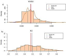
Figure 4 Performance Evaluation Measures for the random forest based downscaling models. a) RMSE and, b) R2.
Table 6 Performance Evaluation Measures for spatial downscaling Models
| Metric | RMSE | R2 | MAE |
|---|---|---|---|
| Mean | 0.043 | 0.492 | 0.0345 |
| Median | 0.043 | 0.476 | 0.0340 |
| Standard deviation | 0.046 | 0.346 | 0.0418 |
The scatter plots and error statistics (Figure B1 and Figure 4) indicate that the downscaling approach using random forest successfully captured the nonlinear relationship between soil water content and the covariates used, particularly at smaller scales (lower spatial resolutions). All models exhibit similar behavior in terms of RMSE, with fluctuations around 0.040 to 0.045 cm3 cm-3 and occasional peaks of up to 0.050 cm3 cm-3. It is evident that on average, RMSE is higher during the wet season (from November to March) and decreases to values around 0.04 cm3 cm-3 for models trained during the dry season (from May to September). Generally, the RMSE falls within the expected accuracy limits of the SMAP product (0.04 to 0.06 cm3 cm-3) (Chaubell, 2016). Thus, having a mean RMSE of 0.043. the evaluated downscaling models possess a suitable capacity for capturing the SMAP soil moisture and predictive covariates relationship.
Figure 4.b shows the coefficient of determination R2, it generally falls within a range of 0.2 to 0.8, indicating relatively good performance of each model in predicting SMAP soil moisture data based on the set of covariates at the original spatial resolution. Regard the temporal distribution of model’s R2, lower R2 values are observed during the dry season (0.20 to 0.30), while higher values are seen during the wet season (~0.40). This behavior is unexpected; typically, models are expected to perform better during dry periods, as demonstrated in numerous previous studies (Wakigari & Leconte, 2022). One possible explanation, reinforced by subsequent results, is that soil moisture distribution becomes more complex during dry periods as well as the inclusion of DEM derivatives in our work that have been demonstrated to be strong predictive factors of soil moisture at basin scale, especially in wet season (Raduła et al., 2018). Distribution during these periods relies less on precipitation and more on subsurface flows, heavily influenced by soil properties that exhibit greater variability at larger scales than topographical or hydrological properties in the landscape (Famiglietti et al., 2008).
This result may seem somewhat discouraging at first glance, but it is only slightly inferior to previous studies (Beck et al., 2021), and there are two specific reasons that can be conjectured: Firstly, the downscaling models were not fully optimized, as explained in the previous section. Secondly, the coefficient of determination (R2) is calculated at the original resolution of the SMAP product. Therefore, it is not a metric solely representing disaggregation error but also reflects the modeling error at those spatial scales.
While it's true that the models should be trained to minimize error and maximize explained variance (R2), the actual predictive capacity of the models is determined by the quality of the covariates and the number of observations available. The models need to strike a balance between optimizing their parameters and the constraints posed by the covariates and observational data, which can influence the models' ability to make accurate predictions.
3.3 Soil moisture Spatial Predictions
Once the models were evaluated and their ability to capture nonlinear relationships between covariates and SMAP soil moisture was ensured, they were applied to the downscaling of soil moisture at high spatial resolutions (~100 m). We generated high resolution soil moisture maps over the studied region using the trained models. For generating the maps, we used all available predictor covariates at their original spatial resolution in a sequential way.
To analyze the predictions in greater detail we show a set of predictions on a small sub-basin located near Cusco City (Figure 5). This figure depicts the process of downscaling of SMAP soil moisture in an area around the monitoring station at the K'ayra weather station through different spatial resolutions for a specific date as an example of the high-resolution soil moisture mapping approach. The white areas represent impermeable surfaces such as urban areas or superficial water bodies, which were excluded from the analysis beforehand.
Figure S1 in Supplement material shows the spatial distribution of daily downscaled soil moisture for Kayra watershed, primarily determined at this resolution by hydro-topography and soil properties. The daily dynamics of soil moisture, primarily influenced by precipitation, can also be observed. The downscaling scheme's capability allows for observing the variability of water flow processes in the soil and their redistribution at high spatiotemporal scales. in soil moisture content). After careful evaluation, it can be postulated that the reason is that the models for those dates were trained with few SMAP pixels, possibly due to non-optimal retrieving conditions. This led to predictions within a covariate range with low variability, resulting in the observed artifacts. This is noticeable in the map generated using the model trained on August 12, 2021.
Certain spatial discontinuities can be observed in some maps from Figure S1 (regions with abrupt changes.
3.4 Spatial Analysis of downscaled soil moisture
The analysis of downscaled soil moisture spatial mean and standard deviation is shown though a Violin diagram in Figure 6.a and 6.b. Figure 6.a demonstrate the high spatial variability of soil moisture during dry and rainy seasons. Additionally Figure 6.b shows a slightly more variability of soil moisture in wet season compared against dry season. This phenomenon has been previously described in studies such as Famiglietti et al., (2008), Mohanty et al. (2017), and Western and Blöschl (1999). The findings of this study are consistent with the moisture dynamics described by the aforementioned authors. Additionally, the study area is significantly large, and it is expected that there would be soil moisture variability, primarily due to precipitation gradients. Considering that each block was sampled within a single pixel of the original 9 km resolution SMAP product, and the sampling was done without replacement, a reasonable representation of moisture distribution for the original 9 km SMAP pixels was obtained.
Based on the analysis of Figure 6.b, it appears that at 100 m resolution the downscaled product is unable to capture the natural spatial variability of soil moisture within 1 km² areas (average standard deviations of 0.05% for both hydrological seasons). Moreover, it seems to be insensitive to the influence of saturation conditions (i.e., both dates exhibit the same standard deviation despite significantly different saturation conditions). This inherent variability in soil moisture (i.e., the spatial variability of soil moisture is considered greater during wet periods) is well-documented in numerous previous studies (Vergopolan et al., 2021). In general, it can be postulated that this is the reason why the subsequent PCA analysis struggled to produce coherent results for the spatial standard deviation of downscaled soil moisture content (σ2DWS).
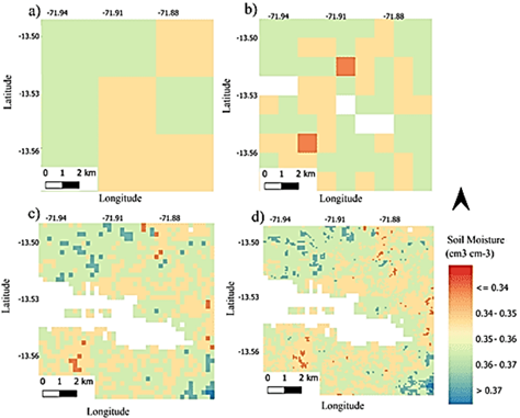
Figure 5 Downscaling of SMAP soil moisture product. a) 3 km, b) 1 km, c) 250 m and d) 100 m spatial resolution near Cusco City.
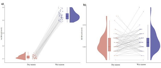
Figure 6 Violin diagrams of downscaled soil moisture mean and standard deviation. a) spatial mean of downscaled soil moisture (μDWS) and b) spatial standar deviation of downscaled soil moisture (σ2DWS) within 1 km2 squared spatial unit randomly sampled over the studied region. Wet season is February 9, 2022, and dry season is August 18, 2021.
3.5 Factors Related to the Spatial Distribution of downscaled soil moisture
Figures 9.a and 9.b displays biplots of principal component analysis for the covariates, both for August 16, 2021, and February 9, 2022, illustrating their relationship with the spatial mean of the downscaled product (μDWS) within 1 km2 squared spatial units randomly sampled over the studied region show in Figure 7.
In general, there is an observable trend in the spatial mean of the downscaled soil moisture in the wet season (February 9, 2022) (Figure 9.b), denoted as μDWS. This tends to follow the first principal component (PC1), which is positively influenced by the variables μDEM and μOC, while being negatively influenced by μDA and μARC (higher clay content and bulk density result in lower μDWS, and higher mean elevation and organic carbon content lead to higher μDWS.
In the dry season, the distribution patterns of soil moisture are not as strong (Figure 7.b), and there is a higher variability not fully explained by the covariables. However, a trend along PC1 is still observable, although the variables no longer explain the moisture distribution as effectively. 𝜌DEM and μKsat are still responsible for high soil moisture values, as well as μMAM, but there is generally more heterogeneity or randomness in the soil moisture distribution. Furthermore, it appears that PC2 better modulates the average soil moisture, particularly the variation in elevation 𝜌DEM, the mean soil sand content μARN, μAlpha, and the saturated hydraulic conductivity μKsat, which seem to modulate moisture conditions in dry periods.
The interpretation of the biplot from Figures 7.a and 7.b allows us to analyze the relationship between downscaled soil moisture and the environmental factors that determine its spatial variability. It is noticeable that soil moisture follows the spatial precipitation gradients of the PISCO product. Points with higher μDWS values are associated with higher μMAM and μDEF values, indicating that the historical mean precipitation described by PISCO during the months of December to May explains the distribution of areas with high soil moisture content. The second principal component is negatively dominated by σDEM and μKsat, and positively by μfd8 and μmd. This implies that higher elevation variability and greater mean saturated hydraulic conductivity of the soil result in lower average soil moisture. Additionally, higher spatial variability of topographic moisture indices leads to higher average soil moisture. However, PC2 can only explain 13% of the total variability of the variables, making its explanatory power for soil moisture variability less than that of PC1.
Soil heterogeneity and its properties, such as texture, organic matter content, bulk density, and saturated hydraulic conductivity, influence the water storage capacity of soils, as well as the speed of flow and redistribution of moisture. This, in turn, contributes to the spatial heterogeneity of the average downscaled moisture, in agreement with prior studies (Brocca et al., 2017; Crow et al., 2012; Famiglietti et al., 2008). In areas with shallow groundwater, such as wetlands (Guevara & Vargas, 2019), this soil heterogeneity plays a much more complex role, requiring additional analysis supported by hydrological models and groundwater level monitoring data. For instance, Warner et al. (2021) achieved excellent results in SMAP downscaling using the KNN model in the CONUS monitoring network (United States), except in wetland-dominated areas, where the model consistently underestimated soil moisture (Guevara & Vargas, 2019). Furthermore, topograph ical and hydrological characteristics, such as surface elevation and topographic wetness index, modulate soil moisture variability towards convergence areas through surface flow/runoff or subsurface lateral flow. The results exhibit high soil moisture variability related to topographic moisture indices μfd8 and μmd, and their spatial variability σfd8 and σmd, illustrating the role of topography in moisture distribution (Beven & Freer, 2001; Liu et al., 2020; Raduła et al., 2018), particularly during wet periods of the year (Western & Blöschl, 1999).
In fact, the results suggest that high-altitude locations (greater μDEM) with high hydro-topographic divergence conditions (low μfd8 and μmd) and low variability (low σfd8 and σmd), along with soils high in organic matter content (greater μOC and μOCS), are associated with higher soil moisture conditions in the study area.
3.6 Field validation
Figure 8 depicts the daily time series of soil moisture in-situ measurements, downscaled soil moisture product, and the difference between them (i.e., 𝜃 𝐸𝑅𝑅𝑂𝑅 ). A strong agreement between the analyzed time series can be observed. The agreement from May to August is nearly perfect, with differences ranging between 0.01 to 0.05 cm3 cm-3.
Figure 8 shows clearly, that starting from October, the downscaled product consistently underestimates soil moisture content, with notable differences ranging between 0.15 to 0.25 cm3 cm-3. This underestimation is particularly significant in November. From December onward, the time series tend to converge, and the differences decrease again to values close to 0.05 cm3 cm-3. After April, the downscaled product tends to overestimate soil moisture content in the validation pixel where the monitoring station is located, resulting in negative differences between the time series in this period (-0.05 cm3 cm-3).
The MQCC analysis allowed for an examination of the relationship between the time series. The following observations can be made from Figure S3. At weekly temporal aggregation levels (graining ~ 7), the correlation between DWS and OBS is strong. At larger time aggregations (14 days ≤ grainings ≤ 20 days), the correlation coefficient decreases, fluctuating between 0.60 and 0.69.
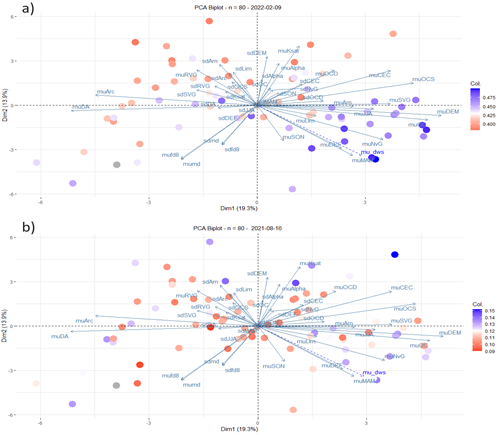
Figure 7 Biplots from PCA analysis. a) Biplot diagram for the covariables for the wet season (February 9, 2022) and their relationship with the spatial mean of downscaled soil moisture (μDWS) within 1 km2 squared spatial units randomly sampled over the studied region. b) Biplot diagram for the covariables for the dry season (August 16, 2022). Axis represents the two first principal components. Prefix mu means spatial mean and prefix sd means spatial standar deviation.
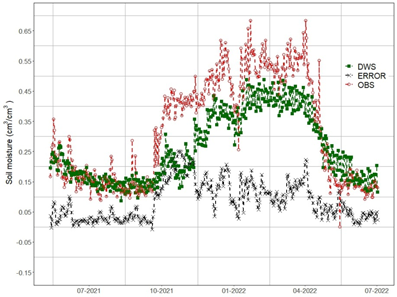
Figure 8 Time series of observed and downscaled soil moisture. DWS represents the downscaled soil moisture product at a spatial resolution of 100 m. OBS refers to the moisture content observed in the field through daily monitoring using the ThetaProbe ML3 sensor within a pixel of the downscaled product. The variable ERROR is calculated as the difference between OBS and DWS, i.e., ERROR = 𝜃 𝐷𝑊𝑆 − 𝜃 𝐹𝐼𝐸𝐿𝐷 .
Additionally, it was expected that the correlation coefficients would vary significantly at different quantile levels (for instance, that the correlation would be higher at quantile τ = 0.1 than at quantile τ = 0.9). The scatter plot suggest that the correlation is higher under low saturation conditions (small quantiles) and lower under high saturation conditions (large quantiles). However, the behavior of the relationship between DWS and OBS at different quantiles remains consistent and independent of the value of τ. For instance, both at τ = 0.1 (considering low saturation values of OBS and DWS time series) and at τ = 0.9 (considering high saturation values of OBS and DWS time series), the regression coefficient fluctuates between 0.65 and 0.95, mod ulated solely by the temporal aggregation scale.
These results are consistent with previous research. For example, Hu et al. (2020) obtained correlations between 0.246 and 0.705 when disaggregating SMAP data for 30 stations in Mongolia. Abbaszadeh et al. (2019) obtained correlation coefficients between 0.65 and 0.70 when disaggregating SMAP data for 300 soil moisture monitoring stations across the CONUS network in the United States. Wakigari & Leconte (2022) obtained correlation coefficients between 0.68 and 0.83 in their study area located in the northeastern region of the United States. Huang et al. (2020) validated a quantile-based random forest (QRF) SMAP downscaling strategy across various monitoring networks worldwide, obtaining correlation coefficients between 0.754 and 0.632. Shangguan et al. (2024) generated downscaled soil moisture data which exhibited satisfying accuracy (mean R = 0.52 and RMSE = 0.047 m3 m3), Sishah et al. (2023) downscaled SMAP soil moisture in small watershed in Ethiopia, following that, the accuracy of downscaled soil moisture against a sensor network was 0.1320 cm3 cm3 Root Mean Square Error (RMSE). Nadeem et al. (2023) gap-filled SMAP soil moisture data, their approach showed high R (0.40) and low RMSE (0.064 m3 m3) against in situ SM.
Singh et al. (2019) which is the most comparable study, as both studies only utilized a single soil moisture sensor, unlike other studies that employed sensor networks, found correlation coefficients ranging from 0.416 to 0.943. Additionally, some studies also analyzed the correlation relationship with land cover, finding that moisture content was better explained by models in pastures (𝜌 = 0.696) than in cultivated areas (𝜌 = 0.624), forests (𝜌 = 0.611), or bare soil (𝜌 = 0.433).
Figure 9 displays the scatter plot between the daily observations of the SMAP downscaled product and the field-observed soil moisture for approximately 400 days.
Regarding the scatter plot in Figure 9, there is an accumulation of points in the low moisture zone (0.1 to 0.2 cm3 cm-3), indicating the overall average moisture for the area. The red regression line diverges from the perfect 1:1 relationship line as moisture increases. It can be observed that the product underestimates observed moisture at higher soil water content values. The distribution of points is quite similar to that obtained by Singh et al. (2019), showing a concentration of points in the low to intermediate moisture range (0.10 to 0.20 cm3 cm-3).
3.7 Methodological limitations
Unlike previous studies such as Abbaszadeh et al. (2019) and Wakigari & Leconte (2022) that parameterized random forests using all available data for an entire study period, this study used approximately 1300 SMAP pixels within the study area. While this approach captures dynamic relationships between soil moisture and covariates, this strategy reduces the sample size used for training the daily models; posing the risk that the models may not have enough observations to effectively capture the relationships between covariates and soil moisture of the SMAP product. This is a challenge observed in machine learning models and is common (Adab et al., 2020; Heuvelink et al., 2021).
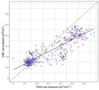
Figure 9 Scatter plot pf observed and downcaled soil moisture. DWS (the downscaled soil moisture product at a spatial resolution of 100 m), OBS (soil moisture observed in the field through daily monitoring using the ThetaProbe ML3 sensor).
In some cases, downscaling models exhibited suboptimal behavior due to lack of hyper-parameter optimization, attributed to computational limitations. Instead of focusing on optimize the models’ parameters, we focused on independent validation through in-situ soil moisture monitoring. In a recent study, (Hernandez-Sanchez et al., 2020; Singh et al., 2019) validated the SMAP product through in-situ monitoring with sparsely distributed sensor network measurements. In the aforementioned studies, a soil moisture measurement station was utilized for each pixel of the SMAP product. This work adopts the subsequent results as a working hypothesis. Therefore, despite potential errors arising from the limited spatial representativeness of soil moisture measured by a single monitoring station, the relationship between in-situ soil moisture and remote estimation was considered acceptable. Additionally, due the lack of in situ analytical soil information spatially distributed at the sub-basin level we choose to use geospatial information for soil physical and chemical properties using the SoilGrids (Hengl et al., 2018) product developed by ISRIC as a covariate. While this enables to use soil properties as predictive variables which can lead to better downscaling results, SoilGrids were not validated for our study region, hence possibly introducing some bias in the results.
4. Conclusions
The present work aimed to assess a machine learn ing technique called random forest to enhance the spatial resolution of remote soil moisture estima tions from the SMAP product of the SMAP satellite for the period from 2015 to 2022. Furthermore, it sought to evaluate these predictions over a hydro logical year in a study watershed.
After training downscaling models using random forest as the downscaling function, it was demonstrated that the temporal disaggregation (reconstruction of time series) adequately captures the temporal dynamics of the SMAP product. Regarding the spatial downscaling, the statistical analysis of RMSE indicated that the generalization error of the downscaling models is suitable for scientific and practical applications (less than 0.05 cm3 cm-3). In conclusion, it was demonstrated that random forest is capable of spatial downscaling of the SMAP product in the study area.
By applying Principal Component Analysis (PCA) to the mean of high-resolution soil moisture and hydrotopographic and soil covariates in 80 systematically sampled polygons within the study area, it was demonstrated that at high spatial resolutions (~ 100 m) and under conditions of moderate to high soil moisture, the downscaled soil moisture product primarily depends on elevation, soil organic carbon content, clay content, and saturated hydraulic conductivity of the soil. Under conditions of lower soil water content, its distribution becomes more random and ceases to depend directly on the covariates used in this study. As for precipitation, it explains the majority of the spatial dynamics of the SMAP product at the original resolutions (~ 9 km).
Through scatter plot and Multiscale Quantile Correlation Coefficient (MQCC) analysis, it has been demonstrated that the time series of the downscaled soil moisture product at 100 m and the time series of soil moisture observed in the field through monitoring with dielectric sensors over 400 days exhibit a coherent and highly significant relationship with each other. More specifically, it can be concluded that the soil moisture downscaled using the random forest model adequately explains the in-situ soil moisture measurements in the monitored area under conditions of low soil moisture content. However, the relationship diverges from this behavior in conditions with moisture contents between 0.4 and 0.5 cm3 cm-3. As a result, the downscaling scheme proposed in this study did not yield satisfactory results under extremely wet (saturation) conditions. Furthermore, at coarse temporal aggregations (approximately weekly averages), the quantile-based correlation coefficients between the time series average around 0.98, regardless of the season. This indicates that the downscaled soil moisture product using random forest explains the in-situ measurements almost perfectly at weekly time aggregations.

