1. INTRODUCTION

Recently, the vision of structural engineering as a discipline have started to change.

Civil structures have also been a fundamental part of any society around the world. Buildings, bridges, and other structures are all necessities for the general population. The loss of any main civil structure can have fatal consequences on economy, social and cultural impacts, and time and life losses. As civil engineering and structural design continue to change and evolve, smart perspectives on the analysis, design and subsequent performance of civil structures must also be transformed. New civil structures must be able to withstand natural hazards, ensure occupant safety, and remain operational after the event¹.

Structural control shows great potential for reducing vibrations in civil structures under any dynamic loading. It can be classified by the type of device used to produce control forces. The three general kinds of structural control devices are passive, active, and semiactive². Semiactive control devices seems to be more appropriate for field applications since they offer the reliability associated with passive control devices, maintain the versatility associated with active control devices and only need a low-power supply³. Many semiactive control devices have been proposed for structural control of civil structures. According to⁴ the magnetorheological (MR) fluid damper appears to be a particularly promising type of semiactive control device. In semiactive control the damper force is controlled in real-time with the goal of improving performance and reducing unwanted responses of the system. In addition to the controllability, stability, low-power requirements inherent to semiactive devices, MRDs, with their large temperature operating range and relatively small device size, have the added benefits of: producing large control forces at low velocities and with very little stiction; possessing a high dynamic range; and having fewer moving parts. Complementary, a total implementation considers a semiactive control strategy. Since semiactive control devices are inherently stable (in a bounded input-bounded output sense), high authority control strategies may be designed and implemented, which in practice, may result in performances that can even surpass that of an actively controlled structure. In this research, a control algorithm based on Lyapunov's stability theory is used⁵.

As explained in⁶, Simulink is defined as a block diagram environment for multidomain simulation and Model-Based Design. It supports system-level design, simulation, automatic code generation, and continuous test and verification of embedded systems. Simulink provides a graphical editor, customizable block libraries and solvers for modeling and simulating dynamic systems. It supports linear and nonlinear systems, modeled in continuous-time, sampled time, or hybrid of the two. It is integrated with MATLAB, enabling to incorporate MATLAB algorithms into models and export simulation results to MATLAB for further analysis.

The focus of this research is to model MRDs for its subsequent use in the semiactive control of civil structures under seismic loading. One of the main challenges to ensure a successful implementation of MRDs is the ability to recreate the physical behavior of the simulated portion of a test with sufficient accuracy so that compatibility can be guaranteed between the simulated and experimental components during testing.

2. BACKGROUND

2.1 Magnetorheological Damper Models

A great effort has been made to develop models that identify the hysterical behavior of MRDs. According to⁷, existing models can be classified into two main categories: non-parametric models, in which the parameters of the models do not necessarily have physical meanings, and parametric models, in which the parameters of the models have some physical meaning. Two models are used and depicted here.

2.1.1 MRD Bouc-Wen Model

The first model of MRD used here corresponds to the modified Bouc-Wen model (BWM), proposed in⁸. A representative schema of the mechanical model is shown in Figure 1.

Fig. 1 MRD Bouc Wen Mechanical Model.⁸. 

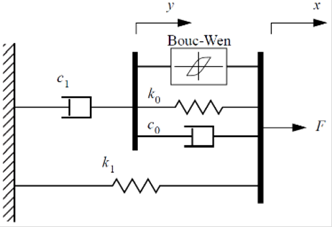
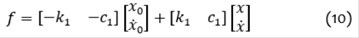
In the description made in⁸ of the proposed BWM, it is found that the governing differential equations of the mechanical model are,

where f represents the force produced by the MRD, k₁ represents the stiffness of the accumulator; c₀ represents the viscous damping observed at high speeds; c₁ was included in the model to reproduce the reduction observed at low speeds; k_o represents the stiffness at high speeds; x_o is the initial displacement of the spring k₁ associated with the nominal force of the MRD due to the accumulator and z is the evolutionary variable of the Bouc-Wen element.

For the sake of the Bouc Wen mechanical model being able to capture the behavior of the MRD, the model had to represent fluctuating current levels. For this purpose, certain parameters had to be modeled as functions of the current; then, three parameters were identified as functions of the current,

where i is the current applied to the MRD.

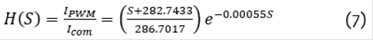
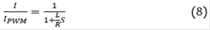
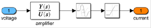
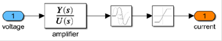
The complementary part, corresponding to the dynamics of the width modulated amplifier (PWM), the dynamics in the magnetic coils and the surrounding MR fluid of the damper, expressed in the frequency domain, is specified below.

Then, a total of 20 parameters were established for the Bouc Wen model (Table I).

TABLE I Bouc Wen Model Parameters. ⁸. 

Parameter	Value	Parameter	Value	Parameter	Value	Parameter	Value
α_A	687.7 kN	c_0B	0.113 kN⋅seg/m	c_1A	100 kN⋅seg/m	β	3000 m^(-1)
α_B	0.006 kN	c_0C	-109 kN⋅seg/m	c_1B	1500 kN⋅seg/m	γ	3000 m^(-1)
α_C	-697.6 kN	c_0D	-2.116 kN⋅seg/m	k_0	0.0559 kN/m	A	336.56
α_D	-0.91 kN	L_0	0.8 H	k_1	0.0641 kN/m	η	2
c_0A	201.3 kN⋅seg/m	L	2 H	x_0	0.01 m	R	4.8 Ω

2.1.2 MRD Hyperbolic Tangent Model

The Hyperbolic Tangent model used in this research is based on the model proposed in⁹. In the description referring to Figure 2, it is found that the Hyperbolic Tangent model is composed of two linear viscous dampers and two springs, which are connected by means of an inertial mass element. The inertial mass element resists movement by means of a Coulomb friction element.

Fig. 2 MRD Hyperbolic Tangent Mechanical Model.⁹. 

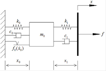
According to⁹, the dynamics of the system and control force can be described in the form of a state space formulation shown in equation 9.

Here, the control force f produced by the MRD is a function of the state in equation 9, the displacement, and the velocity through the damper.

The Hyperbolic Tangent model requires seven parameters (k₀, k₁, c₀, c₁, m₀, f₀ and V_ref) in order to fully identify its dynamic behavior (Table II), where i represents the current entering the MRD.

TABLE II Hyperbolic Tangent Model Parameters.⁹  

Parameters as a function of the damper current (A)	Units
k_0=(0.10i^4-1.00i^3+1.30i^2+2.30i+6.20) 10^(-4)	kN⋅mm^(-1)
k_1=-2.43i^4+23.76i^3-80.70i^2+110.62i+55.08	kN⋅mm^(-1)
c_0=(-0.98i^4+9.33i^3-29.96i^2+35.80i+12.64) 10^(-2)	kN⋅seg⋅mm^(-1)
c_1=(0.62i^4-6.73i^3+26.69i^2-46.06i+35.67) 10^(-2)	kN⋅seg⋅mm^(-1)
m_0=(0.16i^4-1.62i^3+5.48i^2-7.05i+4.85) 10^(-3)	kg
f_0=1.52i^4-10.27i^3+2.79i^2+94.56i+6.19	kN
V_ref=-0.12i^4+1.36i^3-6.19i^2+13.12i+0.76	mm⋅seg^(-1)

The complementary part, corresponding to the dynamics of the width modulated amplifier (PWM), the dynamics in the magnetic coils and the surrounding MR fluid of the damper, is similar to the Bouc Wen model.

2.1.3 System of Governing Differential Equations

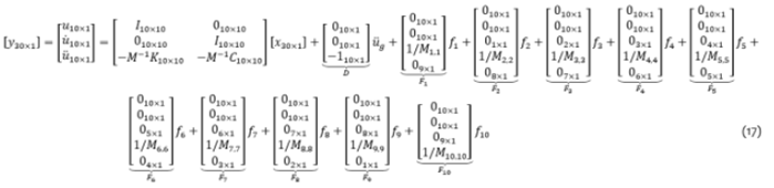
According to¹⁰, when considering a building model under seismic excitation controlled by n MRDs and assuming that the control forces are adequate to maintain the structural response in the linear region, the set of differential equations of motion governing the control system can be written compactly as shown in equation 11,

where M is the mass matrix, C is the damping matrix, K is the stiffness matrix, 1 is a column vector with all elements equal to 1, ü_g is the acceleration component of the ground used, f is the force vector control and Λ is a matrix determined by the location of the MRDs in the structure.

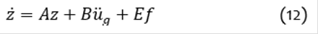
Equation 11, after a representation procedure in the form of state spaces, corresponds to the arrangements of equations 12 and 13, where z is the vector of states and y is the vector of outputs.

2.1.4 Structural Control Algorithm

The actions of active, passive, semiactive and hybrid structural control systems are based on the excitation and/or responses of the structure¹⁰. The calculation of the appropriate control action is based on the control algorithm that maps the input (input signals) to the output (control signals). When this mapping is linear, the controller is linear and when the map is non-linear, it is referred to as a non-linear control algorithm¹¹. Therefore, the control algorithm plays a transcendental role in the performance of the control system.

As established by¹², the expression 14 corresponds to the calculation of the voltage or current of the ith MRD in a control system,

where V_máx is the maximum applied voltage or current, H(·) is the Heaviside step function, f_i is the force produced by the ith MRD, z is the vector of states of equations 12 and 13 and E_i is the vector of the ith column of matrix E in equation 12.

The calculation of the matrix P in equation 14 requires the previous establishment of the matrix Q_P and the solution of equation 15,

known as the Riccati equation. A challenge in using the algorithm based on Lyapunov's stability theory is the selection of an appropriate Q_P matrix.

3. METHODOLOGY

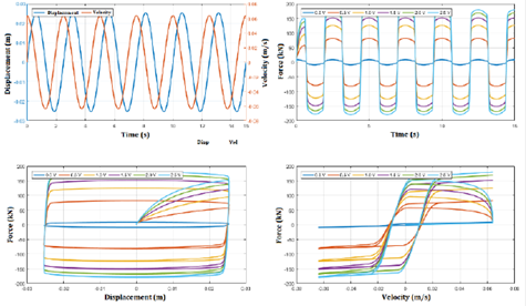
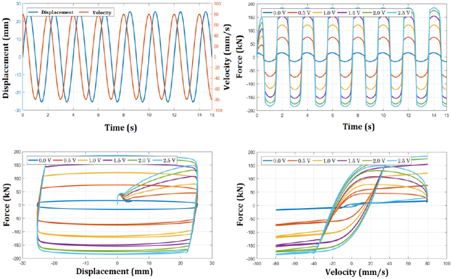
First, the modeling of the MRDs (Bouc Wen and Hyperbolic Tangent models) were aimed at replicating the laboratory results obtained in⁴ and illustrated in part here.

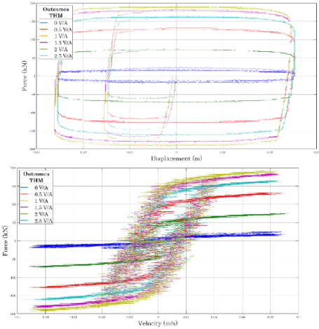
Fig. 3 Graphical representations Displacement vs. Force & Velocity vs. Force. (MRDs laboratory results).⁴. 

Next, a semiactive control system including a semiactive control strategy, MRDs, and an idealized frame with ten degrees of freedom was established. Finally, the input of the system corresponds to a record of ground accelerations and the outputs correspond to displacements, velocities and accelerations at various frame levels according to equation 13.

3.1 Modeling of the MRD Bouc Wen model

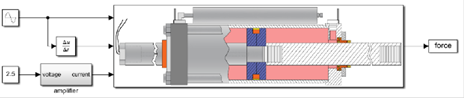
The Simulink block diagram was established according to the representative expressions of the mathematical model and parameters shown in the theoretical framework. (In detail in¹³).

Fig. 4 Main Simulink block diagram for the Bouc Wen Model.¹³. 

Fig. 5 Simulink block diagram for the Amplifier PWM.¹³. 

Fig. 6 Simulink block diagram for the governing differential equations.¹³. 

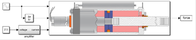
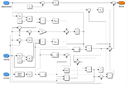
The results of the simulation of the main Simulink block diagram of the Bouc Wen MRD (Figure 4), for different values of voltage or current (similar to those in the laboratory test⁴), are shown in the graphs below.

Fig. 7 Graphical representations. (MRDs research results).¹³. 

3.2 Modeling of the MRD Hyperbolic Tangent model

The block diagram was established in Simulink according to the representative expressions of the mathematical model and parameters shown in the theoretical framework. (In detail in¹³).

Fig. 8 Main Simulink block diagram for the Hyperbolic Tangent Model.¹³. 

Fig. 9 Simulink block diagram for the Amplifier.¹³. 

Fig. 10 Simulink block diagram for the governing differential equations.¹³. 

The results of the simulation of the main block diagram of the Hyperbolic Tangent MRD (Figure 8), for different values of voltage or current (similar to those in the laboratory test⁴), are shown in the graphs below.

Fig. 11 Simulink block diagram for the governing differential equations. [13] 

3.3 Modeling of the structural control system

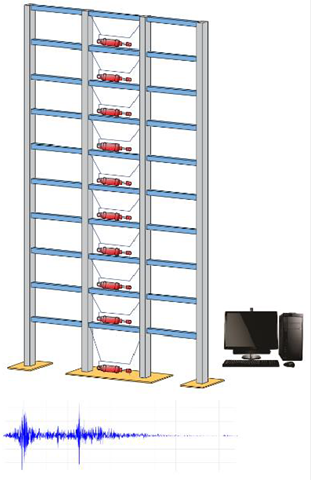
A representative image of the control system to be implemented is shown in Figure 12. This system is composed of an idealized frame with 10 levels, 10 magnetorheological dampers, a computer and a ground acceleration component.

Fig. 12 Implemented Semiactive Control System.¹³. 

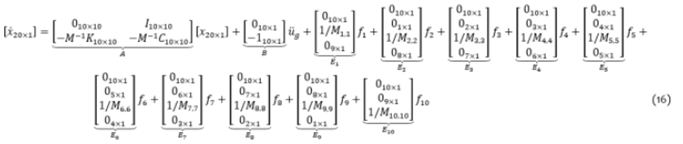
An important point is the matrix development of the control system to be implemented, whose description through the formulation of state spaces is shown in equations 16 and 17. (In detail in¹³).

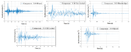
In order to test the control algorithms implemented in this research, five records were selected to perform time-history analyses of the building model under seismic excitations (Figure 13):

• El Centro. The N-S component recorded at the Imperial Valley District Irrigation Substation in El Centro, California, during the Imperial Valley earthquake on 05/18/1940.

• Hachinohe. The N-S component registered in the city of Hachinohe during the Tokachi-oki earthquake on 05/16/1968.

• Northridge. The N-S component recorded in the parking lot of the Sylmar County, California hospital during the Northridge earthquake on 01/17/1994.

• Kobe. The N-S component recorded at the Japanese Kobe Meteorological Station (JMA) during the Hyogo-ken Nanbu earthquake on 01/17/1995.

• Pisco. The N-S component registered at the San Luis Gonzaga National University station in Ica, during the Pisco earthquake on 08/15/2007.

Fig. 13 Ground acceleration records used in this research.¹³. 

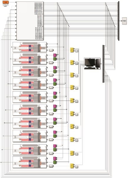
The main semiactive control system is shown in Figure 14. It consists of a closed loop system and contains more than 1000 Simulink blocks (In detail in¹³). First, this system is used to establish the Q_P matrix of equation 15, according to the acceleration records used in the present research.

Fig. 14 Implemented Semiactive Control System by Simulink block diagram.¹³. 

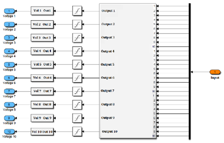
A representative block diagram of the implemented semiactive control algorithm is shown in Figure 15. It corresponds to the display of the block with a computer image of Figure 14. (In detail in¹³).

Fig. 15 Implemented Semiactive Control Algorithm by Simulink block diagram.¹³. 

4. RESULTS

The main achievement of the present research was to establish the modeling and simulation of a structural control system with MRDs for the reduction of the structural response in buildings using MATLAB and Simulink. The problem was characterized, first, by modeling the magnetorheological dampers based on mechanical models with established parameters and its subsequent validation based on experimental results. Then, buildings under seismic excitation were modeled, in order to obtain the response that it is desired to reduce. Finally, the structural control systems with magnetorheological dampers were also modeled.

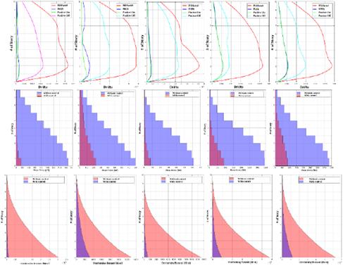
According to the implemented control system and the ground acceleration records, the results corresponding to the story drifts, shear forces and overturning moments are presented below (Pisco, Hachinohe, Northridge, El Centro and Kobe), illustrating the reduction proposed at the beginning of the research.

Fig. 16 Graphical representations (Pisco, Hachinohe, El Centro, Northridge and Kobe).¹³. 

CONCLUSIONS

The main conclusions of the research are:

The implementation of the Simulink block diagram for the Bouc Wen and Hyperbolic Tangent MRD mechanical models could be carried out programmatically using the MATLAB Fcn block¹⁴. The implementation in block diagram, in general, is due to the computational efficiency in relation to the simulation time of the model.

Upon obtaining results from the simulation of the block diagrams that represent mechanical models of Bouc Wen and Hyperbolic Tangent MRDs, the research continued making use of the Hyperbolic Tangent MRD based on the fact that this model has more recent studies that implement the dynamics in the magnetic coils and the MR fluid. Additionally, by means of a statistical analysis of the Displacement vs. Force and Velocity vs. Force graphs (experimental and mathematical model), it was inferred that the use of the tanh function in the Hyperbolic Tangent model (shown in Figure 17) exhibited the numerical results (plotted in Figure 11) in a more adequate way in relation to the experimental results (plotted in Figure 3). The implementation of other mechanical models that represent MRDs can be done in the same way and with knowledge of what was implemented in the Bouc Wen and Hyperbolic Tangent models here.

The key point in the establishment of Simulink block diagrams for controlled and uncontrolled systems is the development of arrangements called state space formulation, which in turn interacts in a very similar way with Simulink's StateSpace block¹⁴. In the uncontrolled case, the State-Space block had a single input that corresponded to the acceleration component of the soil used, and, in the controlled case, the ground acceleration and the control forces produced by the MRDs were considered as inputs.

Simulink has a variety of solvers that can be set or chosen automatically¹⁴. The ode45 solver used in the present research did not present any drawbacks in the simulation using a step size of 0.001. Additionally, the ode45 solver is, generally, the first choice that must be taken into account.

The establishment in a block diagram of the control algorithm based on Lyapunov's theory came to be determined after several simulations of the control systems, because there is no pattern to determine the Q_P matrix that intervenes in the calculations.

The establishment of the Simulink block diagrams that represent the structural control system was carried out taking into account a MRD for each floor, as a consideration of systems for research purposes and not for real practice. It should be noted that the number of MRDs, the location in the system, and the ability to generate control forces are current research topics.

Based on the fact that the response of a building is evaluated by its story drift, shear forces and overturning moments, it was possible to establish results showing the reduction in graphical form. The first and fundamental results corresponded to the reduction of displacements, which caused a reduction in story drifts, shear forces and bending moments.

The reduction of displacements, velocities and accelerations at the level of the first floor was achieved, with the reduction of displacements being the most significant and the reduction of accelerations the least significant; thus, confirming what is established in the revised literature.