


 Inglés (pdf)
 Articulo en XML
 Referencias del artículo
 Enviar articulo por email
 Citado por SciELO
  Similares en
SciELO
Similares en
SciELO 
 Permalink
1. INTRODUCTION
In Peru, procedures of pavement design are based on a simplified, but costly, assumption, which is that soils in the subgrade would eventually become completely saturated in their service life. However, not all regions of the country will have fully saturated subgrades. Field evidence and numerous numerical modeling studies have shown that, although the pavement acts as a covering of unbound material, the water content of the subgrade will change over time [1]. For this reason, there is a need to study design methodologies that allow us to consider the subgrade in its unsaturated state. In the state of the art of pavement design there are methodologies, such as the empirical-mechanistic guide of AASTHO, which considers the unsaturated behavior of the subgrade soil. Unfortunately, this type of methodology is not yet applicable in Peru, because they require dynamic equipment, such as the cyclic triaxial, to determine the resilient modulus, tests to measure soil suction, and an extensive registry of climate information that are not yet available [2]. Due to this, even in our country we continue to use the saturated CBR test to estimate the bearing capacity of the subgrade, a condition that according to Kodikara et al. [3] is very conservative and recommends that detailed evaluations of the humidity variation in the field should be carried out to make more rational pavement designs. A methodology that does not require sophisticated equipment that allows estimating the bearing capacity (CBR) of the soil in its unsaturated condition is the spectrum of RAMCODES (Rational Methodology for Compacted Geomaterial's Density and Strength Analysis) design curves [4], which its author created with the purpose of designing compacted soils and, thus, optimize their properties. However, this methodology has not yet been adequate to be used in the design of pavements and, thus, be able to consider the unsaturated behavior of the subgrade soil. For this reason, this research will try to answer the following question: How can the spectrum of RAMCODES design curves be implemented in the design of flexible pavements in order to consider the behavior of unsaturated soils? A problem of great relevance since, if solved, it could be optimized in the conformation of the pavement layers.
Finally, the objective of this research is to implement the RAMCODES design curve spectrum of unsaturated subgrades of silty clayey sands to the design of a flexible pavement considering the environmental and traffic conditions of section 1 of the Oyón-Ambo highway.
2. BACKGROUND
In 2012 Sánchez-Leal [4] presents a tool of the RAMCODES methodology which is called RAMCODES design curves. This methodology is based on three topics: soil mechanics, statistics, and weight-volume relationships. For the construction of the design curves, the author proposes the execution of laboratory tests under a factorial experimental approach, where the independent variables are the water content and the compaction energy, and the dependent variable is the response of the soil (hydraulic properties or mechanical properties). In addition, examples are presented of how the use of this methodology offers advantages in both safety and economy.
Feo and Alvarado [5], in 2012, used the RAMCODES resistance map for quality control in cohesive soil embankment construction. For the elaboration of the resistance map, a test embankment was built with a silt-clayey soil, selected for the conformation of the core of a dam. The variables used for the elaboration of the map were dry unit weight, water content and undrained shear strength. It was concluded that the use of RAMCODES resistance maps allows analyzing trends and understanding complex behaviors, such as undrained shear resistance, useful information for rapid control of embankments in the field, allowing confidence in the release of compacted layers.
Oyola-Guzmán and Oyola-Morales [6] in 2018 used the design curves of the RAMCODES methodology to explain the cause of failure of a compacted soil, whose compaction quality control was only verified by the minimum percentage of compaction (95% of the maximum dry unit weight of a standard proctor or a modified proctor). The design curves were obtained from the results of the laboratory tests of a silt-clayey sand where its water content and dry unit weight were varied, and the mechanical response of the soil was measured based on the CBR test. It was concluded that the failure occurred because the minimum compaction percentage criterion was used, a criterion that is not sufficient to predict the performance of a soil against loads, since the mechanical response of the soil is not considered.
3. METHODOLOGY
3.1 ESTIMATION OF THE VARIATION OF SATURATION AND PHYSICAL-MECHANICAL PROPERTIES
To carry out this research, the environmental conditions of section 1 of the Oyón-Ambo highway were taken into consideration; so, the variation of subgrade soil saturation had to be estimated. To do this, historical information on daily rainfall in the Oyón region for a period of 20 years had to be compiled. This information was obtained from [7], and with this data, the maximum daily rainfall was obtained. After this, a mathematical model (1) developed in [8] was used to predict the variations of the daily volumetric water content from the maximum daily rainfall, but the initial volumetric water content was modified to the volumetric water content corresponding to the optimum water content and a degree of compaction of 95% of the maximum dry unit weight. This was done to adjust the mathematical model to the conditions of our case study. In addition, these variations were estimated at a depth of 0.7 m from the subgrade soil and the analysis will be conducted at this depth according to the recommendations in [9].
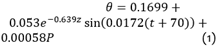
Where θ is the volumetric water content (cm3/cm3), z represents the depth of analysis (m), t is the time since January 1 (days) and P is the maximum daily precipitation (mm).
Thus, with the volumetric water content data obtained, their respective degrees of saturation were calculated using (2). In this calculation, a dry unit weight of 95% of the degree of compaction of the subgrade soil was considered. Finally, the monthly saturations of the subgrade were obtained at a depth of 0.7 m by averaging the daily saturations of each month.

Where Sr is the degree of saturation (%), Gs is the specific gravity of soil solids, γω is the specific weight of water (g / cm3), γd is the dry unit weight of the soil (g / cm3) and θ is the volumetric water content (cm3 / cm3).
In addition, a 1.5 m deep test pit was made at the side of the road section under study to characterize the subgrade soil in physical-mechanical terms. Three hundred kilograms of soil were extracted and transported to the city of Lima to be tested in the CISMID geotechnical laboratory. A series of tests were performed on the subgrade soil under ASTM standards, which are mentioned in Table I.
TABLE I. ASTM standards used to obtain the properties of the subgrade soil
To compare the results obtained with the subgrade characterization methodology used in this research (RAMCODES design curve spectrum), a conventional CBR test will be performed, i.e., a test where three CBR specimens previously submerged in a pond for 4 days are penetrated, and the final curve reported (which relates dry unit weight and resistance (CBR)) as USACE CBR curve, since this procedure is suggested by the U.S. Army Corps of Engineers (USACE) [9].
3.2 CONSTRUCTION OF THE SPECTRUM OF RAMCODES DESIGN CURVES
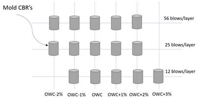
To construct the spectrum of RAMCODES design curves, the first thing that was carried out was a CBR factorial experiment under the alternative stipulated in section 4.2.2 of [10], where it is mentioned that CBR tests can be carried out where not only the compaction energies as is usually done, but also the water contents. Since this standard does not mention in detail how to carry out this variant, we will rely on [11]. The steps followed to perform the CBR factorial experimental are listed below:
a. The modified proctor test was performed according to [12].
b. Fifteen soil specimens were made by compacting each specimen in five layers of pre-wetted soil material, using a given number of blows of the 4.5 kg proctor hammer and using the 15 cm diameter mold.
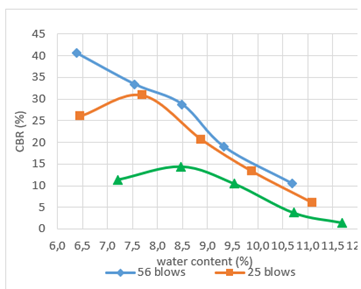
c. The fifteen specimens were divided into three groups according to the compaction energies 56, 25 and 12 blows per layer, as shown in Fig. 1.
d. Specimens for 56 blows/layer were made with moistures of OWC-2%, OWC-1%, OWC, OWC+1% and OWC+ 2%.
e. Specimens for 25 blows/layer were prepared with moistures of OWC-2%, OWC-1%, OWC, OWC+1% and OWC+ 2%.
f. Specimens for 12 blows/layer were prepared with moistures of OWC-1%, OWC, OWC+1%, OWC+2% and OWC+ 3%.
g. Each specimen was tested in the CBR press at the compaction moisture and placing the preset number of overloads.
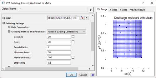
Likewise, the information obtained from the CBR factorial test was processed using a statistical program called OriginPro 2019b. The steps followed to obtain the RAMCODES design curve spectrum are listed below:
a. The data obtained from the CBR factorial experimental were entered into a new worksheet in the program.
b. The data entered was converted into a matrix network using a gridding method. Sánchez-Leal recommends using the random correlation kriging type gridding method under the configuration of columns, rows, search radius, maximum and minimum points and smoothing shown in Fig. 2.
c. A three-dimensional surface (response surface) and a contour map (resistance map) were generated from the data of the matrix network with the "plot" option.
d. A new worksheet was created to enter a range of water content to obtain the saturation curves from (3).
e. The saturation curves entered were added to the contour map created.
f. The intersections of the saturation curves and the contour map were noted on an Excel sheet.
g. The RAMCODES design curves were plotted from the data recorded on the Excel sheet.

Where ɣd is the dry unit weight of the soil (g/cm3), ɣω is the specific density of water (g/cm3), ω is the water content (%), Gs is the specific gravity of soil solids, and Sr is the degree of saturation (%).
3.3 DETERMINATION OF EFFECTIVE RESILIENT MODULUS AND CRITICAL RESILIENT MODULUS
For the determination of the effective resilient modulus, we rely on Chapter 2 (design requirements) of [13]. This chapter details how to obtain the effective resilient modulus based on the seasonal resilient modulus. In the present research, the procedure was adapted so that the RAMCODES design curves can be implemented to obtain the seasonal resilient modulus. The adapted procedure is detailed below:
a. The RAMCODES design curves were interpolated to obtain the resistances (CBR) of the soil in its unsaturated state considering the monthly saturations in the subgrade at a depth of 0.7 m and that the soil has a density equal to 95% of the maximum dry unit weight.
b. From these seasonal (monthly) CBRs, the seasonal resilient moduli were obtained using (4).
c. The relative damage corresponding to each seasonal resilient modulus was calculated and the average relative damage was obtained.
d. With the average relative damage and using (5), a resilient modulus was calculated, which is called effective resilient modulus.
In [13] it is emphasized that this effective resilient modulus should be used only for the design of flexible pavements based on serviceability criteria.

Where Mr is the resilient modulus (psi) and CBR is the California Bearing Ratio

Where μf is the relative damage and Mr is the resilient modulus (psi).
On the other hand, the critical resilient modulus was also estimated, which would represent the subgrade soil in its saturated condition. To obtain the aforementioned modulus, we used the USACE CBR curve. Through this curve, we obtained the CBR of the soil for a density equal to 95% of the maximum dry unit weight. Finally, from the CBR value, the critical resilient modulus was obtained using (4).
3.4 EVALUATION OF THE DESIGN OF A FLEXIBLE PAVEMENT
To evaluate the structural contribution of considering the subgrade in its unsaturated state, two flexible pavement designs were carried out based on the pavement design methodology described in [14], which in turn is based on [13]. The first design considered the effective resilient modulus (obtained through the RAMCODES design curve spectrum) and the second the critical resilient modulus (obtained through the USACE CBR curve).
For the pavement design, the projected traffic for 20 years for section 1 of the Oyón-Ambo highway was considered, which was calculated in [15]. In addition, the values of standard deviation (Zr), combined standard error (S0), initial serviceability index (PSI0) and final serviceability index (PSIt) were taken from the recommendations of [14]. The structural number (SN) of the pavement was obtained by means of (6). As it can be seen in this equation, it is not possible to solve it by clearing the value of SN; therefore, an iterative process must be followed by means of some algorithm of approximation of the zeros.
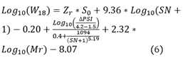
Where W18 is the projected 18 kip (18000 lb) equivalent load number of simple axial load application (ESAL), Zr is the normal standard deviation, S0 is the combined standard error of projected traffic and projected performance, △PSI is the difference between initial serviceability index (PSIo) and terminal serviceability index (PSIt), Mr is the resilient modulus (psi) and SN is the structural number indicative of the total pavement thickness required.
After calculating the value of SN, the thicknesses of the flexible pavement were obtained by means of (7). It should be noted that the pavement components and their respective layer coefficients were extracted from [14] and [15].

Where SN is the structural number indicative of the total pavement thickness required, D1 is the thickness of the wearing course (cm), a1 is the structural layer coefficient of the wearing course (cm), D2 is the thickness of the base course (cm), a2 is the structural layer coefficient of the base course (cm), m2 is the drainage coefficient of the base course (cm), D3 is the thickness of the subbase course (cm), a3 is the structural layer coefficient of the subbase course (cm) and m3 is the drainage coefficient of the subbase layer (cm).
Finally, the pavement layer thicknesses obtained by using the effective resilient modulus versus the critical resilient modulus were compared.
4. RESULTS
4.1 ESTIMATION OF THE VARIATION OF SATURATION AND PHYSICAL-MECHANICAL PROPERTIES
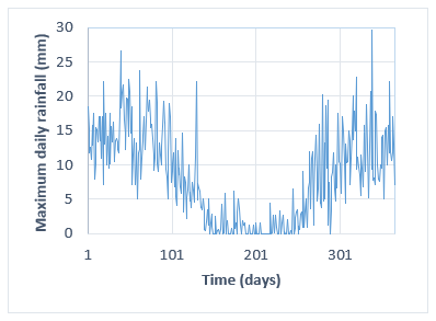
The maximum daily rainfall for a period of twenty years (1994-2013) is shown in Fig. 3. It can be seen that the dry season goes from May to September and the wet season goes from October to April, which is consistent with that described in [15]. The maximum precipitation found in this period was 29.6 mm, the minimum was 0 mm, and the average precipitation was 8.2 mm. A period of twenty years was considered because of the lifetime of the pavement under study.
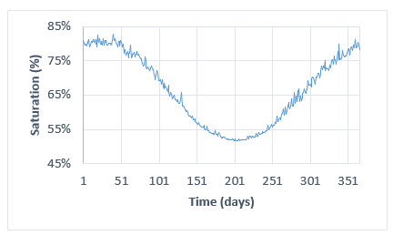
By means of (1) and (2) the variation of daily saturations was obtained from the maximum rainfall in the subgrade at a depth of 0.7 m. Fig. 4 shows the results that follow the same trend as the rainfall (Fig. 3). The maximum saturation found was 82.8% while the minimum was 51.8%. According to [8], one of the limitations of the model used is that it does not consider the heterogeneous stratigraphy, so it could not be used for subgrades with different layers. Currently, there is another more generalized methodology to estimate the variation of moisture in the subgrade, which is called Enhanced Integrated Climatic Model (EICM), but according to [2] the access to the climatic information required by EICM in our country is very restricted, due to its high cost, and mainly because there is no need to accumulate climate information according to the needs of this methodology. Therefore, it was decided to use the mathematical model developed in [8].
Based on the estimation of the daily variations of saturation in the subgrade, we proceeded to obtain the variation of the monthly average saturations. These results are shown in Table II. While some authors, as in [8], mention that the saturation of the soil in the subgrade varies over its lifetime, other authors, as in [1], mention that the soil reaches a constant equilibrium saturation if the water table is relatively deep. Something that should be taken into account is that the variation of saturation will be strongly influenced by the quality of the drainage system of the pavement; however, the presented estimates of the variation of saturations may not be the true ones, but they give us an estimate of how it would behave for the conditions studied in [8].
TABLE II Monthly average variation of saturation in the subgrade
| Month | value |
|---|---|
| January | 80.4 |
| February | 79.6 |
| March April May June July August September October November December | 75.4 68.1 60.5 54.6 52.1 53.3 58.4 65.6 72.7 77.9 |
In the 1.5 m test pit that was excavated, a continuous silty clayey sand stratum was found, with a percentage of fines of 29.8%, sands of 59.6% and gravel of 10.6%. Table III shows a summary of the results of the tests performed in the geotechnical laboratory of CISMID. It can be seen that the natural field moisture was lower than the optimum water content by 0.45%.
TABLE III Physical properties of subgrade soil
| Soil properties | value |
|---|---|
| Liquid limit (%) | 23 |
| Plastic limit (%) | 17 |
| Plasticity index of soils (%) | 6 |
| Water content (%) SUCS classification AASTHO classification Specific gravity of soil Optimum water content (%) Maximum dry unit weight (g/cm3) | 8.1 SC-SM A-2-4 (0) 2.68 8.55 2.09 |
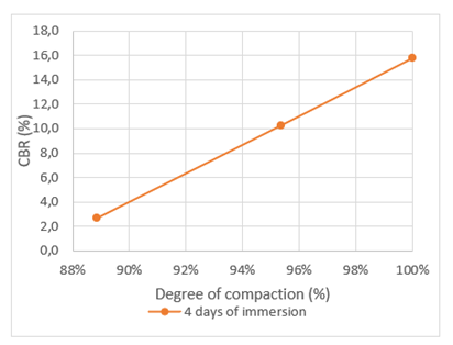
Fig. 5 shows the USACE CBR curve, which was obtained from a CBR test under four days of immersion. With this curve, it is possible to find the CBR at different degrees of compaction of the subgrade soil. In our case study, a subgrade compacted to 95% of the maximum dry unit weight was considered; therefore, the CBR of the subgrade under this methodology is 10%. However, this methodology assumes that in four days of immersion, the soil inside the mold will be saturated. A consideration that is not verified, also according to [10], is that the molds prior to their penetration should be inclined to let the water drain for a period of fifteen minutes, which would generate that the suction in the soil increases in an uncontrolled manner, so the USACE CBR curve would not provide us with results for a saturated condition.
4.2 CONSTRUCTION OF THE SPECTRUM OF RAMCODES DESIGN CURVES
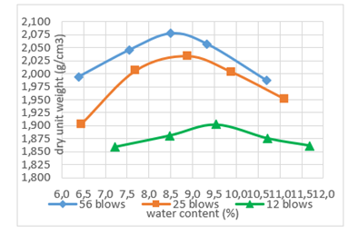
The compaction curves obtained by means of a CBR factorial experimental are shown in Fig. 6. It can be seen that these curves follow the trend described in [16], in which it is mentioned that as the compaction energy increases, the maximum dry unit weight will also increase and also the optimum water content will be reduced to a certain extent. Likewise, Fig. 7 shows the CBR resistance curves, where it is evident that as the compaction energy increases, the resistance of the soil also increases. However, if we observe both figures together, we can see that the highest strengths do not occur when the soil has a dry unit weight equal to the maximum and a water content equal to the optimum, but occur when the soil has a water content lower than the optimum. However, these results are not anomalous, but follow the same trend as the results of a factorial CBR experiment performed on a Vicksburg clayey soil shown in [17].
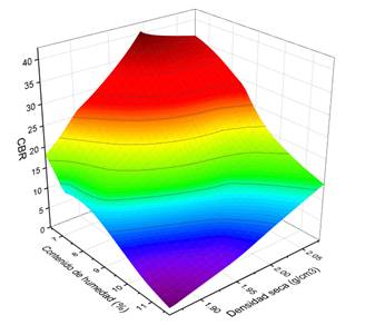
To construct the response surface of the subgrade soil and the resistance map, the results of the CBR factorial experiment shown in Table IV were used. The response surface, shown in Fig. 8, describes the three-dimensional behavior of the water content, dry unit weight and resistance (CBR) of the subgrade soil under study. It can be seen that the minimum resistances of the soil occur when they have high water contents and low resistances, but the maximum resistances do not occur when the soil has the highest density, and this is congruent with what was explained previously.
TABLE IV Results of the CBR factorial experimental
| Number of blows | Water content (%) | Dry unit weight (g/cm3) | CBR - 0.1’’ (%) |
|---|---|---|---|
| 56 blows | 6.38 7.54 8.49 9.33 10.69 | 1.99 2.05 2.08 2.06 1.99 | 41 33 29 19 10 |
| 25 blows | 6.45 7.69 8.88 9.88 11.09 | 1.90 2.01 2.03 2.00 1.95 | 26 31 21 13 6 |
| 12 blows | 7.21 8.48 9.54 10.72 11.68 | 1.86 1.88 1.90 1.88 1.86 | 11 14 10 4 2 |
By means of the resistance map shown in Fig. 9, it is possible to obtain the soil resistance for certain conditions of water content and dry unit weight, but, unlike the response surface, this one is more practical since it is a 2D representation. It is observed that the maximum resistances obtained in this soil are lower than the maximum obtained in the Visksburg clay shown in [17]. This could seem wrong since the soil under study is granular and as it is known, generally granular soils tend to have higher strengths than fine soils. However, as mentioned in [18], this is only true for soils that have water content values higher than the optimum; but, for soils with lower values, the premise is the opposite, i.e. fine soils will have higher strengths than coarse soils and the latter would explain the reason why the Visksburg clay has higher strengths in its dry branch compared to the strengths of the soil under study.
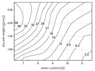
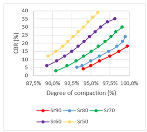
Fig. 10 shows the saturation curves that were plotted on top of the resistance map from (3), using a Gs= 2.68 and saturation degrees of 50%, 60%, 70%, 80% and 90%. By intersecting these saturation curves and the resistance map, the spectrum of RAMCODES design curves was obtained. It is deduced that an infinite number of saturation curves could be obtained, but it would not be practical to plot them all. Therefore, only five saturation curves were drawn to subsequently obtain five design curves.
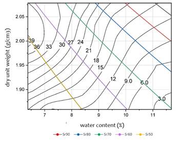
Fig. 11 shows the spectrum of RAMCODES design curves. These curves, unlike the USACE CBR curve, allow us to obtain the resistance of a soil for different degrees of saturation for a given degree of soil compaction. It can be seen an increase in soil resistance when the density of this increases. This is due to the increased contact between particles which generates an increase in friction and consequently in the resistance. It can also be seen that another factor that causes the soil resistance to increase is the decrease in saturation. This last factor can be explained by means of the soil-water characteristic curves, which relate saturation and soil suction in an inversely proportional manner, i.e., when soil saturation decreases, soil suction increases and therefore its resistance [19].
4.3 DETERMINATION OF EFFECTIVE RESILIENT MODULUS AND CRITICAL RESILIENT MODULUS
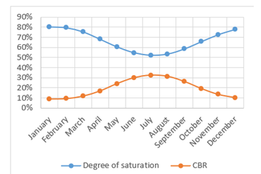
By means of the monthly variation of saturation in the subgrade at a depth of 0.7 m and the RAMCODES design curve spectrum for a density equal to 95% of the maximum dry unit weight, it was possible to obtain the monthly (seasonal) variations of the resistance (CBR) of the soil. Fig. 12 shows the monthly variation of the saturation and the resistance of the subgrade soil. It can be observed that the soil has the minimum resistance in January due to high soil saturation and a maximum resistance in July due to low soil saturation.
The seasonal resilient moduli obtained from the CBRs by means of (4) are shown in Table V. This correlation was chosen because it is still recommended in an appendix of the empirical-mechanistic design guide [20]. In addition, it can be seen that the change of the resilient modulus due to saturations varies proportionally to the values of the empirical model relating these variables developed by the NCHRP 1-37A project [18]. On the other hand, some authors, as in [21], mention that Mr-CBR correlations should be used with caution because they tend to "over-predict" or "underestimate" the resilient modulus. In this regard, the best method to determine the resilient modulus is by means of a cyclic triaxial equipment, but unfortunately in our environment there is no operative one available.
TABLE V CBR and seasonal resilient moduli
| Month | CBR (%) | Mr (psi) |
|---|---|---|
| January February Mach April May June July August September October November December | 8.9 9.2 11.7 16.8 24.1 29.9 32.4 31.2 26.1 19.1 13.4 10.3 | 10327.2 10600.8 12357.4 15562.1 19564.1 22458.8 23677.1 23120.1 20614.9 16897.4 13440.6 11334.0 |
Table VI shows the relative damage corresponding to each seasonal resilient modulus. The average of these relative damages is 0.02657 and, by means of (5), we obtain an effective resilient modulus equal to 14401.6 psi. This effective resilient modulus will represent the bearing capacity of the road under study for a period of twenty years considering the variation of saturation in the subgrade due to the maximum rainfall that may occur in the study area.
TABLE VI Relative seasonal damage
| Month | Mr (psi) | Relative damage |
|---|---|---|
| January February Mach April May June July August September October November December | 10327.2 10600.8 12357.4 15562.1 19564.1 22458.8 23677.1 23120.1 20614.9 16897.4 13440.6 11334.0 | 0.0575 0.0541 0.0379 0.022 0.0131 0.0095 0.0084 0.0089 0.0116 0.0183 0.0312 0.0463 |
On the other hand, from the CBR obtained by means of the USACE CBR curve, the critical resilient modulus was also calculated and a value equal to 11153.0 psi was obtained. This critical resilient modulus would represent the bearing capacity of the road under study in a critical saturation condition (close to 100%). However, this condition is not met because the CBR test under four days of immersion fails to saturate the soil completely (as already explained in section 2 of results). accordingly, the verification of the saturation that the subgrade reached for the resistance (CBR) that corresponds to 95% of the degree of compaction was performed using the USACE CBR curve and it was obtained that the soil in this condition reached a saturation of 78.3% far from 100% that is intended to simulate this methodology. For this reason, by obtaining the bearing capacity of the subgrade under the aforementioned curve, we would be estimating its value under a saturation of less than 100% and which is not verified, which would lead to unreliable pavement designs.
TABLE VII Relative seasonal damage
| Layer | Structural coefficient (1/cm) | Drainage coeffici ent |
|---|---|---|
| Asphalt road | 0.17 | ------------ |
| Surface | ------------- | |
| Base | 0.052 | 1.00 |
| Subbase | 0.047 | 1.00 |
When comparing the resilient modulus obtained, we observe that the effective resilient modulus is higher than the critical resilient modulus by 29%. This increase is explained by the fact that, to obtain the effective resilient modulus, we take into account the unsaturated behavior of the subgrade soil.
4.4 EVALUATION OF THE DESIGN OF A FLEXIBLE PAVEMENT
This section shows the variation obtained when using an effective resilient modulus calculated by the RAMCODES design curves versus the critical resilient modulus obtained by the USACE design curves in a flexible pavement design. Table VII shows the design parameters used for the calculation of the pavement structural number under the AASTHO 93 methodology. It is observed that the structural number obtained considering the effective resilient modulus is lowered by 8.4% compared to considering the critical resilient modulus, which will be reflected in a reduction of thicknesses in the pavement layers.
TABLE VIII Relative seasonal damage
| Parameter | Critical Mr | Effective Mr |
| W18 | 6.9E6 | 6.9E6 |
| Zr | -1.282 | -1.282 |
| S0 | 0.45 | 0.45 |
| PSI0 | 4 | 4 |
| PSIt | 2.5 | 2.5 |
| Mr (psi) | 11153.0 | 14401.6 |
| SN req. | 3.93 | 3.60 |
The materials used to form the flexible pavement are presented below:
a. Roadbed: hot mix asphalt mat (HMA), with an elastic modulus of 2965 MPa (430 Ksi) at 20°C (68°F).
b. Base: granular base with CBR equal to 80% compacted to 100% of the maximum dry unit weight.
c. Subbase: granular subbase with CBR equal to 40% compacted to 100% of the maximum dry unit weight.
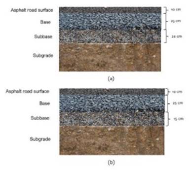
The structural layer and drainage coefficients of each pavement layer are shown in Table VIII, which were extracted from the recommendations of [14] and [15]. From these values of layer coefficients, the thicknesses of the flexible pavement were calculated. For both resilient moduli, the minimum values recommended in [14] were considered for both the thickness of the asphalt layer and the base; so, the thickness to be calculated will be that of the subbase. When the critical resilient modulus was used, a subbase thickness of 20 cm was obtained, and when the effective resilient modulus was used, a thickness of 15 cm was obtained, which represents a decrease in the subbase layer thickness of 25%. Therefore, the hypothesis of this research is accepted, which considered that the implementation of the RAMCODES design curve spectrum of unsaturated soils to the design of a flexible pavement allows us to optimize the pavement thicknesses, considering the environmental and traffic conditions of section 1 of the Oyón-Ambo highway. The final thicknesses of the flexible pavement calculated by both resilient moduli are shown in Fig. 13.
TABLE IX Flexible pavement layer coefficients
| Layer | Structural coefficient (1/cm) | Drainage coefficient |
|---|---|---|
| Asphalt road surface | 0.17 | --------------- |
| Base | 0.052 | 1.00 |
| Subbase | 0.047 | 1.00 |
CONCLUSIONS
A procedure is established to implement the RAMCODES design curves for unsaturated soils in the design of flexible pavements considering the environmental and traffic conditions of section 1 of the Oyón-Ambo highway.
The subgrade soil was a silty clayey sand, with 29.8% fines, 59.6% sand and 10.6% gravel, with a liquid limit equal to 23%, plastic index of 6%, specific gravity of 2.68, optimum water content of 8.55% and maximum dry unit weight of 2.09 g/cm3. Likewise, it was possible to estimate the variation of saturations in the subgrade for a period of twenty years at a depth of 0.7m, by means of a mathematical model adapted to the conditions of the case study. This proved, in an approximate way, that the saturation in the subgrade did not have a value close to 100%, but that its value fluctuates throughout its lifetime.
It was observed that the greatest resistances do not occur when the soil has a dry unit weight equal to the maximum and a water content equal to the optimum, as is commonly believed, but they occur when the soil has a water content lower than the optimum. However, these results are not anomalous, but follow the same trend as the results of a CBR factorial experimental done on a Vicksburg clay soil, and this is due to an increase in soil suction when its water content is decreased.
Based on a CBR factorial test, varying the compaction energies and soil water contents, the RAMCODES design curve spectrum was constructed from a range of saturations between 50% and 90%. The method specified in AASTHO 93 design guide was adapted to obtain the effective modulus of the subgrade by means of the aforementioned curve spectrum.
From two designs of flexible pavements, by traditional methodology of subgrade characterization and the one proposed in this research. By considering the unsaturated behavior of the subgrade, the pavement design is optimized because the resilient modulus of the subgrade increased by 29% and the thickness of the pavement layers was reduced by 25%, especially the thickness of the subbase layer.

