


 Inglês (pdf)
 Artigo em XML
 Referências do artigo
 Enviar este artigo por email
 Citado por SciELO
  Similares em
SciELO
Similares em
SciELO 
 Permalink
1. INTRODUCTION
The Peruvian subduction zone has generated giant megathrust earthquakes. The great historical 28 October 1746 event affected Central Peru destroying Lima, with an estimated moment magnitude of 8.8 [1]. A similar event has not occurred since then, however, Villegas-Lanza et al. [2] estimated for Central Peru, using interseismic coupling models, a Mw 8.7-8.8 event. Therefore, Lima is in constant threat by the occurrence of a big event.
In the last 20 years, Peru has experienced a consistent growth of infrastructure, mainly focused in Lima, its capital. In this city, according to a recent study of the Peruvian Chamber of Construction (CAPECO) [3], constructed area has increased from 1.96 million of m2 in 2002 to 4.97 million of m2 in 2020, with a peak of 6.98 million of m2 in 2014. Construction in the residential sector concentrated 85% of the total constructed area in the year 2020, representing 4.22 million of m2. Social housing contributed with 1.67 million of m2, promoted trough the MiVivienda Fund of The Ministry of Housing, Construction and Sanitation of Peru, with the new MiVivienda credit and Techo Propio program. In addition, CAPECO [4] shows preferences for living in buildings has increased gradually since 2002. Recently constructed, residential buildings Tempo (Urbana Peru Inmobiliaria) and MET (Senda Inmobiliaria) are 37 stories height. However, the average number of stories is not uniform in Lima. It varies from the minimum of 6.7 in North Lima and the maximum of 13.9 in Downtown Lima as pointed by CAPECO [4].
As a part of the aforementioned growth, in North Lima, in the district of Comas, a project with more than 100 buildings, so far, have been constructed progressively for the last 10 years. Buildings range from 12 to 16 stories with 6 to 8 apartments per floor. Depending on the block, typical architectural and structural design has been used. In order to satisfy both productivity in construction and interstory drift limits imposed by Peruvian standards, in high urban density projects with identical mid-rise buildings, reinforced concrete shear walls are used as lateral load resisting system.
On the other hand, after a big earthquake hits, questions arise regarding the capacity of structures to resist aftershocks following the main event. Inspection of infrastructure is crucial in order to prevent people to expose their lives in a possible building collapse. Engineers would inspect buildings one by one taking many days and with the uncertainty of judging as safe buildings where more detailed inspection would have been necessary.
In this context, seismic structural health monitoring presents an opportunity to assess rapidly buildings after a great earthquake and protect a big number of inhabitants from those buildings with high risk of collapse due to aftershocks. Moreover, when identical buildings are part of a residential project, the impact of monitoring just one is greater due to results can represent the behavior of all identical buildings.
2. METHODOLOGY
Seismic response is calculated by instrumentation on different floors of a building and acceleration time histories are recorded. This data needs to be processed in order to understand the dynamic behavior and to obtained useful information for structural health monitoring.
Fourier Transform has been widely used to analyze the frequency content of nonstationary signals. Although, Fourier Transform gives unambiguously the predominant frequencies in a signal, it is not possible to see how they change over time. In response, the Short Time Fourier Transform (STFT), that takes the Fourier Transform of a windowed part of a signal and shifts the windows over the signal [5], and the Multiple Filter Technique (MFT) [6], that applies an array of narrow-band filters to the signal, are used to obtain frequency and time information of a signal. The time-frequency resolution is controlled by a constant window length in the STFT and a constant filter bandwidth in the MFT, however, a constant value for these parameters does not result in same resolution for low and high frequencies. On contrast, wavelet analysis, that is the breaking up of a signal into shifted and scaled versions of the original (or mother) wavelet, allows the use of long time intervals for more precise low-frequency information, and shorter regions for high-frequency information [7]. The wavelet must satisfy the following mathematical criteria: 1) It must have finite energy, 2) It must have a zero mean and 3) For complex wavelets, the Fourier transform must both be real and yet also vanish for negative frequencies [8].
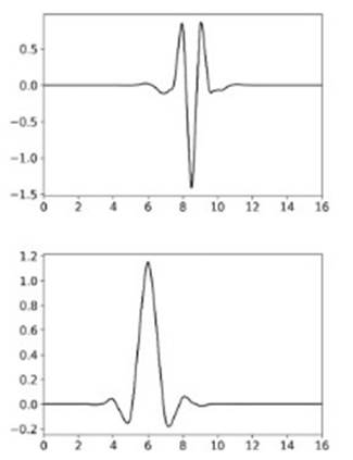
As an example of wavelet, Fig. 1 shows the coiflet wavelet of order 3 and its corresponding scaling function. This avelet has been used for the calculation of the Discrete Wavelet Transform (DWT).
(1)2.1 CONTINUOUS WAVELET TRANSFORM
The Continuous Wavelet Transform (CWT),
The asterisk indicates that the complex conjugate of the wavelet function is used in the transform. This dilation and contraction of the wavelet is governed by the dilation parameter
Equation (2) is the total energy contained in a signal
Equation (3) corresponds to the relative amount of energy related to a specific
The scalogram, as the spectrogram (based on STFT) and the non-stationary spectrum (based on MFT), shows the non-stationary behavior of the signal, however, with the aforementioned advantages. Detecting predominant frequencies and the energy distribution over time is possible.
(4)2.2 DISCRETE WAVELET TRANSFORM
The wavelet function used for the CWT, where
In order to link
where m and n are integers that control the wavelet dilation and translation, respectively.
In practice, the ‘dyadic grid’ arrangement, when
The scaling function is associated with the smoothing of the signal and has the same form as the wavelet, given by
The scaling function can be convolved with the signal to produce approximation coefficients as follows:
We can represent a signal
We can see from this equation that the original continuous signal is expressed as a combination of an approximation of itself, at arbitrary scale index
Hence, the signal
Accordingly, for a discrete signal
Where component signal
The frequency range of the signal component for a specific Rank
2.3 STRUCTURAL HEALTH MONITORING
Observation of dynamic parameters of structures and its variation gives important information about the structural health of buildings. Long-term monitoring for tracking the natural frequency of the building could show fluctuation of this parameter associated to damage that could lead to retrofitting works [11, 12].
Therefore, the main objective is to track natural frequency measured from recorded earthquake at the top of the building. This parameter is obtained from Fourier spectra, Scalograms and Fourier Spectra of the component signal for the predominant response extracted using the DWT. In addition, microtremor measurement at different floors are performed in order to obtain natural frequency. Finally, theoretical fundamental frequency was obtained from a 3D finite element model and an elastic analysis.
3. DESCRIPTION OF THE TARGET BUILDING AND DATA
The building is located in the district of Comas, northern Lima. It is a fifteenth story reinforced concrete shear walls residential building and uses a reinforced concrete mat foundation. Fig. 2 shows the general and top view of the building as well as shear walls distribution and the sensors location whose data were use in this study. Its construction was completed in 2017 and has been instrumented since March 2019.
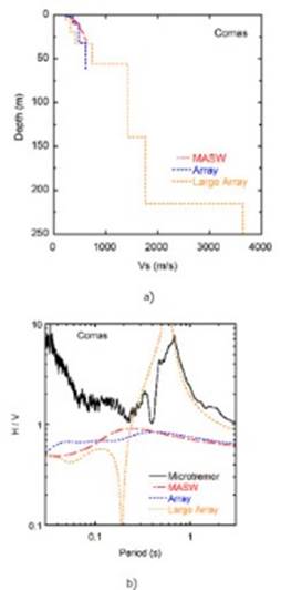
The building rest on deposits characterized as medium dense sands and stiff silts shallow layers follow by medium dense gravel, with average shear wave velocity in the upper 30 m of 420 m/s [13]. Additionally, it is available a deep shear wave velocity (Vs) profile for the location of the building with values of shear velocity larger than 3000 m/s [14]. The strong velocity contrast is the main cause of the particular H/V spectrum shape and the value of fundamental period. Fig. 3 shows the aforementioned deep shear wave velocity and H/V spectrum.
A basic seismic structural health monitoring arrangement is used. It consists of one low-cost sensor called Raspberry Shake 4D (RS-4D, v.6) installed on the roof building level (See filled rectangle in Fig. 2.d). This sensor incorporates both a vertical velocity geophone and three orthogonally positioned microelectromechanical systems (MEM) accelerometers with a sampling frequency of 100 Hz with a flat response up to close to the Nyquist frequency of the sensor (50 Hz). Table I shows main specifications for the sensor reported by the manufacturer (https://raspberryshake.org). Anthony et al. [15] evaluated the performance of three RS-4D (v.5) and found they performed within specifications; however, the MEMs accelerometers have such high noise levels that they are not suitable for studies using ambient seismic noise or teleseismic events. In the present study, it was difficult to extract events from recorded signals with amplitudes close to 1.0 cm/s2 and were not included. Miranda et al. [16] instrumented the fifteenth story SIATA Tower (Medellín, Colombia) with seven RS-4D at different floors and values from 1.0 to 5.0 cm/s2 were reported for four events, however, it is inferred they could not record ambient vibration with the sensors as maximum noise level of 0.05 Gal is suggested for that purpose. On the other hand, CISMID [17] installed a RS-4D in the LIM001 seismic station. From results for an event on April 19, 2021 (Mw 5.0) concluded the signals presented a good approximation, with respect to the signals recorded by a REFTEK 130 SMA sensor installed next to the RS-4D, both in time and frequency domain, however, PGA values from the RS-4D are around 3.80 cm/s2 smaller and a difference in Fourier spectra for short periods is observed.
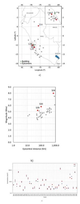
A total of 40 earthquakes between March 2019 and November 2021 have been recorded. Magnitude of earthquakes range from 3.7 to 8.0 (Mw), and epicentral distances from 11 to 884 km. Peak values of horizontal acceleration range from 1.47 to 151.80 cm/s2. Fig. 4 shows Epicenter location of earthquakes as well as moment magnitude versus epicentral distance of the earthquake respect with the building location, and peak values of horizontal acceleration for recorded earthquakes. In Fig. 4, three earthquakes, with greater values of recorded acceleration, are highlighted. They are shown in TABLE II.
In addition, microtremor measurement were performed at first, second, eighth and fifteenth floors (See filled circles in Fig. 2.d) on May 2019. Recording instrument was a three-component seismometer (velocimeter) called Geojar and assembled by Sara Instruments. Measurements were 15 minutes ambient vibration record in each floor and were not simultaneous.
TABLE I Specifications for Rasberry Shake 4D
| Sensor | Samples per second | Flat Frequency Range | Dynamic Range | Noise Level | |
|---|---|---|---|---|---|
| 3-component +/- 2g MEMs sensor (Class C) | 100 | V6+: DC to 44 Hz | 144 dB (24 bits) | 0.3 Gal |
TABLE II Highlighted earthquakes
| Earthquake | Origin local time | Magnitude (Mw) | Depth (km) | Epicentral distance (km) | Peak acceleration (cm/s2) | |
|---|---|---|---|---|---|---|
| X | Y | |||||
| S04 | 26/05/2019 02:41:12 | 8.0 | 135 | 708 | 72.23 | -64.46 |
| S30 | 22/06/2021 21:54:17 | 5.8 | 32 | 95 | 126.23 | -151.80 |
| S39 | 28/11/2021 01:32:30 | 5.2 | 64 | 54 | 64.65 | -70.96 |
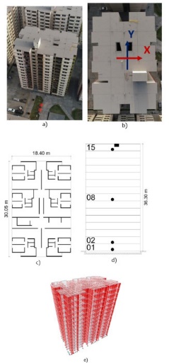
Fig. 2 Target building. (a) General view, (b) Top view, (c) Shear walls distribution, (d) Sensor location and (e) Structural model.
4. RESULTS
Natural frequencies in both directions of the building were obtained from microtremor measurements at different stories. The scalogram from the measurement at fifteenth floor shows energy concentration around 2.0 Hz for both directions for the total duration of the record. Fourier spectra show natural frequencies are 2.19 and 2.04 Hz for X and Y directions (See Fig. 2), respectively. These values have good agreement with those theoretical calculated from a 3D finite element model and an elastic analysis. Microtremor are very small amplitude vibration, in that sense, calculated natural frequencies represent the natural response of the building. TABLE III show values of natural frequencies from microtremor measurements and the structural model. Scalograms and Fourier spectra also show evidence of frequencies for higher mode response.
TABLE III Natural Frequencies (Hz) for microtremor and model
| Direction | Microtremor | Model |
|---|---|---|
| X | 2.19 | 2.03 |
| Y | 2.04 | 1.94 |
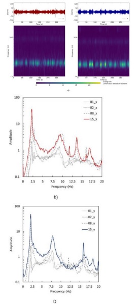
Fig. 5 Results from microtremor measurements. (a) Scalograms in both directions and (b) Fourier spectra in X direction and (c) Fourier spectra in Y directions.
On the other hand, the basic seismic structural health monitoring arrangement does not allow to calculate the response of the building by performing a transfer function between top and base of the building or the structural deformation calculated as the relative displacement between top and base. Therefore, the recorded time histories of earthquakes represent the response of the soil-structure system, hereinafter referred to as the system. Natural frequencies from microtremor measurements are used as a reference due to they are given for small amplitude and represent the natural vibration of the building.
Natural frequencies in both directions of the system were obtained from earthquake recordings at top of the building. Scalograms show energy concentration around 2.0 Hz for both directions. The duration where energy concentrates around this value of frequency is not constant depending on the particular characteristics of magnitude, depth and epicentral for a particular earthquake. An example of the scalogram is shown in Fig. 6 for the earthquake S30 (See TABLE II) where, in addition, Fourier spectra show natural frequencies are 1.93 and 1.81 Hz for X and Y directions (See Fig. 2), respectively. In Fig. 6, Fourier spectra of the record for the earthquake S30 is shown with Fourier spectra of the component signal of the natural response of the system, extracted using the DWT and represented by Rank 5 with frequency range from 1.56 to 3.12 Hz (See (15)). In addition, Fourier spectra of the component signal of Rank 3 with frequency range from 6.25 to 12.50 Hz is also plotted. In general, for recorded earthquakes, scalograms and Fourier spectra also show evidence of frequencies for higher mode response.
A band-pass Butterworth filter between 0.05 to 40 Hz was applied for all earthquake recorded signals.
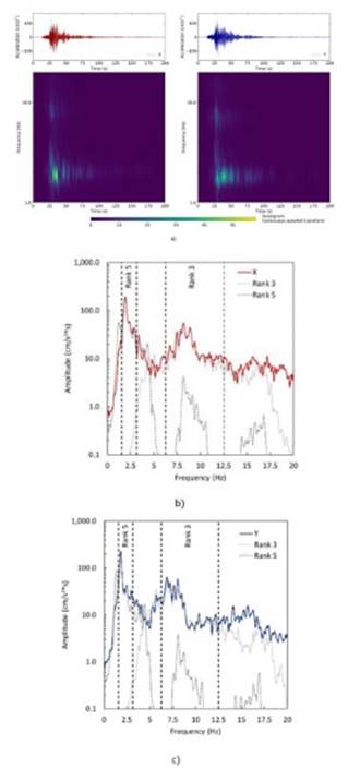
Fig. 6 Results from microtremor measurements. (a) Scalograms in both directions and (b) Fourier spectra in X direction and (c) Fourier spectra in Y directions.
It is observed that natural frequencies for both directions of the system calculated from earthquake records are close to those calculated from microtremor measurements. However, for earthquakes S04, S30 and S39, frequencies present a drop of 5 to 12%. For earthquake S30, with the maximum value of recorded acceleration, frequency value in X direction shifted from 2.19 to 1.93 Hz, where as in Y direction shifted from 2.04 to 1.87 Hz. This drop of frequency is associated with the soil-structure interaction and more sensors are required to study this effect. Fig. 7 shows natural frequencies for earthquakes and acceleration versus natural frequencies.
It was observed that Fourier spectra of Rank 5 represent the natural frequency of the system, as a consequence, it is suitable to look for frequency values using just Rank 5.
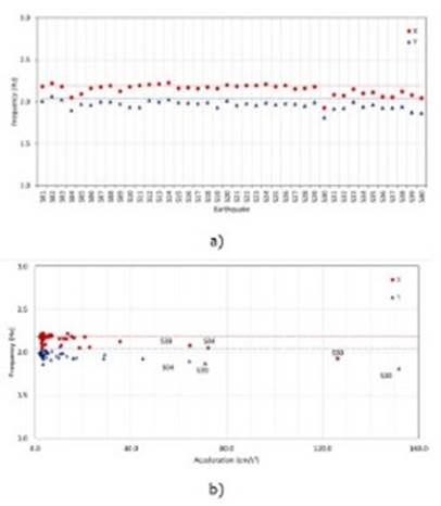
Fig. 7 Natural frequency of building. (a) Natural frequency for earthquakes and (b) Acceleration versus natural frequency.
Calculations were performed using Obspy [18]. Matplotlib [19] and QGIS [20] were used for plots.
CONCLUSIONS
A low cost sensor called Raspberry Shake 4D was deployed on the top of a fifteenth story reinforced concrete shear wall residential building. Forty earthquakes were recorded with a maximum value of horizontal acceleration of approximately 150 cm/s2 for an Mw 5.8 event (S30) with epicentral distance from the building of 95 km. Due to the high noise level of this sensor was not used for ambient vibration measurements.
The continuous wavelet transform has proven an advantage over the traditional Fourier analysis for detecting predominant frequencies and energy distribution over time. In addition, it was possible to decomposed a discrete signal into signal components with a limited frequency range using the discrete wavelet transform.
Natural frequencies in both directions of the building were calculated using microtremor measurements and were validated with the theoretical natural frequencies calculated from a 3D finite element model and an elastic analysis.
It was observed that natural frequencies for both directions of the soil-structure system calculated from earthquake records are close to those calculated from microtremor measurements. However, for earthquakes with greater values of acceleration, frequencies present a drop of 5 to 12%. For earthquake S30, with the maximum value of recorded acceleration, frequency value in X direction shifted from 2.19 to 1.93 Hz, where as in Y direction shifted from 2.04 to 1.87 Hz. More sensors are needed to study the soil structure interaction.

