


 English (pdf)
 Article in xml format
 Article references
 Send this article by e-mail
 Cited by SciELO
  Similars in
SciELO
Similars in
SciELO 
 Permalink
1. INTRODUCCIÓN
The significance of methods for estimating seismic displacements is due to the potential occurrence of large landslides triggered by earthquakes of certain magnitudes, as noted by Keefer [5]: "Moderate to large earthquakes can cause large landslides at great distances from the epicenter, with distances up to 500 km, depending on their magnitude".
Kramer [6] provides a comprehensive explanation of the effects of seismic movements on slopes in his book. Seismic movements generate significant horizontal and vertical dynamic stresses, producing shear and normal dynamic stresses along potential failure surfaces within the slope.
Dynamic shear stresses can exceed the available shear strength of the soil and cause inertial instability on the slope when combined with previously existing static shear stresses. Numerous techniques have been proposed for the analysis of inertial instability, differing in the precision with which seismic motion and dynamic slope response are represented. The subsequent sections describe several common approaches to inertial instability analysis. Pseudo-static analysis, the first approach, calculates a factor of safety along the slope failure surface under seismic conditions, like how static limit equilibrium analyzes factors of safety against static slope failure. All other approaches attempt to assess permanent slope displacements caused by seismic shocks [6].
The importance of the methods for estimating seismic displacements lies in the large landslides that can occur due to earthquakes of a certain magnitude, from the results of Keefer [5]: “The earthquakes of moderate to large magnitude can trigger large landslides at great distances from the epicenter such as 500 km, this depending on its magnitude”.
Due to the different existing methods, it is necessary to evaluate the application of each of these; Fig. 1 shows a diagram of the methods available to analyze a slope in a seismic condition.

2. BACKGROUND
2.2 RIGID BLOCK MODEL
The rigid block model was proposed by Newmark in 1965, based on the simplification of the sliding surface by that of an infinitely rigid block that slides on a flat surface whose movement begins when the accelerations induced by earthquakes exceed the yield acceleration, ky.
During the movement of the sliding block the speed of the support surface and the sliding mass are different, the movement (sliding) will continue until the following 2 conditions are met:
When the accelerations no longer exceed the yield acceleration, ky
The speed of the sliding mass is equal to the speed of the underlying ground or bearing surface.
During each interval of movement of the block, the permanent displacements accumulate, and these will be determined with the double integration method, which consists of obtaining the speed of the block from the integration of the acceleration that exceeds the yield acceleration, ky, as a function of time and then obtain the displacements by integrating said speed as a function of time. The Fig. 2 illustrates the simplification to rigid block model:
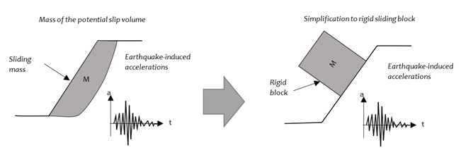
Fig. 2 Representative diagram of the mass simplification of the potential sliding volume to a rigid sliding block.
The theoretical assumptions presented by the rigid block model are described below based on what Murphy [7] mentions in his publication:
The sliding mass is assumed to be a non-conforming or non-deformable rigid block (acceleration of the sliding mass is equal to the acceleration of the bearing surface while “a<ky”, where "a" refers to the acceleration of the sliding mass)
The performance behavior of the material is non-elastic, perfectly plastic (implicit in the use of ky).
The displacements are assumed to occur along a single well-defined slip surface (typically the critical pseudo-static surface of Limit equilibrium method, ky-associated surface)
The material does not suffer loss of strength because of shocks.
The accelerations and the corresponding inertial forces act in the direction of the initial motion at the center of gravity of the sliding mass.
2.1 DECOUPLED MODEL
The decoupled model was proposed by Makdisi and Seed [3], based on the concepts of slip and permanent deformation proposed by Newmark in 1965, but modified by considering the dynamic response of the sliding surface. The dynamic response of this model is the result of the development of codes to perform a finite element analysis. The decoupled model is made up of 2 parts, hence its name:
The dynamic response analysis, which consists of obtaining the dynamic response of the sliding mass as a function of depth, this calculation can be done with one-dimensional or two-dimensional systems, resulting in an average of the accelerations acting on the sliding mass as a function of the time known as horizontal equivalent acceleration, AEH (t).
The sliding response analysis is performed with the double integration of the horizontal equivalent acceleration.
The theoretical assumptions presented by the decoupled model corresponding to the dynamic response analysis are described below based on what Murphy [7] mentions in his publication:
Sliding mass is modeled as a compliant block (if there is a dynamic response).
The dynamic response of the slipping mass is not influenced by the slip that occurs, as these two behaviors are modeled by separate analyzes (the slip surface is not present for the dynamic response analysis).
The nonlinear stress-strain hysteretic behavior of the material is modeled in an approximate way (most commonly linear-equivalent based on iterations).
Seismic waves approximate horizontally polarized and vertically propagating shear waves.
And the theoretical assumptions presented by the decoupled model corresponding to the sliding response analysis are the same as the rigid block mentioned above.
2.3 COUPLED MODEL
The coupled model cannot be attributed to a single researcher since that its use has been proportional to the evolution of numerical codes and the greater computing power available. The coupled analysis is used in sophisticated numerical codes such as FLAC, OpenSees and PLAXIS, although there are also simplified methods based on equations (e.g., Bray and Travasarou [8]). The coupled model manages to represent the interaction between the dynamic response and the slip response that the decoupled model could not relate to.
As can be seen in Fig 3, there are various models for the mechanism of earthquake-induced deformation.

3. METHODOLOGY
3.1 NEWMARK METHOD 1965
Acceleration record acquisition: The seismic accelerations record is collected for the three earthquakes mentioned (Atico 2001, Lima 1974 and Pisco 2007) in the NS and EW directions. The accelerations at the base of the slope failure surface downstream of the dam are obtained.
Evaluation of the threshold acceleration (creep acceleration): The value of the creep acceleration (ky) is determined for the specific case of the dam under study. The creep acceleration has been obtained from a pseudo-static analysis with a factor of safety, SF=1, in this case the value is 0.28 g.
This acceleration represents the available soil resistance that must be overcome for sliding to occur.
Integration of accelerations: The mathematical integration method is used to obtain the velocities; the integration is performed when the acceleration recorded at the base of the slope failure surface exceeds the value of the creep acceleration.
Displacement calculation: Integration is applied again to obtain the total displacement of each of the analyzed columns of the dam.

3.2 SARMA METHOD 1975
Definition of initial parameters: The fundamental period, peak acceleration at the surface and soil depth are determined. These parameters are necessary for the calculation of earthquake-induced deformations.
Calculation of creep acceleration (ky): Using the information provided, the value of creep acceleration (ky) is determined. This acceleration represents the available strength of the soil and is used to evaluate the resulting deformation.
Obtaining earthquake-induced displacements: The algorithm and the figure provided (Fig. 5) are used to calculate the earthquake-induced displacements. Note that Sarma's method considers the frequency content of the ground motion, which distinguishes it from other simplified methods.
Verification of the allowable displacements: The displacements obtained are compared with the established allowable displacements. According to the literature, it is mentioned that the allowable displacements should be less than 1 meter c < 1m).

3.3 MAKDISI & SEED METHOD 1978
Calculation of creep acceleration (yield acceleration, K y ): Using the available data, the value of creep acceleration ( K y ) is determined. This acceleration represents the available resistance of the soil and is an important parameter in the calculation of earthquake-induced deformations.
Calculation ü máx (maximum Acceleration): Using earthquake data and dam geometry, and a nonlinear seismic response analysis, the maximum acceleration at the dam crest is determined.
Use of the 1st abacus (see Fig. 6): The 1st abacus is used to determine the value of K max/ ü máx (coefficient that relates the available resistance to the maximum acceleration at the crest of the dam).
Use of the 2nd abacus (see Fig. 6): Using the values of k y, K max/ ü máx , and the magnitude of the moment of the earthquake ( M w ), the 2nd abacus is used to determine the earthquake-induced displacements.

3.4 METHOD OF BRAY MACEDO AND TRAVASAROU 2018
Determination of the necessary variables: Using the input parameters provided (ky, Ts, 1.5 * Ts, Mw, Sa(1.5Ts)), the values corresponding to each variable are determined.
Calculation of the probability of zero displacements (P (D = 0)): Depending on the value of the fundamental period Ts, the following formulations are applied to calculate the probability that no displacement will occur:


Where ϕ represents the cumulative distribution function of a standard normal distribution.
Estimation of non-zero seismic displacement (D): Using the coefficients a1, a2 and a3 provided in the formulation, the natural logarithm of the estimated displacement (ln(D)) is calculated. The complete formulation is shown below:

Where the values of a1, a2 and a3 are provided in the text, depending on the condition 10sTs ≥ 0 o 10sTs < 0.
a1 = -6,896; a2 = 3,081; a3 = -0.803 for 10 sTs ≥ 0.
a1 = -5,864; a2 = -9,421; a3 = 0.0 for 10 sTs < 0.
The method of Bray, Macedo, and Travasarou [4] is a simplified approach for estimating deformations in dams by considering the sliding mass with a coupled model. This method integrates the dynamic response and sliding response, specifically focusing on subduction earthquakes. The input variables required for the analysis include the yield acceleration (ky), the fundamental initial period (Ts), the degraded period (1.5Ts), the moment magnitude (Mw), and the spectral acceleration (Sa(1.5Ts)). The method provides the displacement along with a probability of non-displacement as the result, which can be considered as a mixed variable.
It is important to follow the exact formulations and make sure you use the correct values for each input parameter. The application of the method of Bray, Macedo and Travasarou [4] will require an analysis of seismic response and spectral adjustment based on the specific data of the rockfill dam with central core, using the acceleration records of the earthquakes (Lima 1974, Atico 2001 and Pisco 2007).
3.5 APPLICABLE CASES: ROCKFILL DAM WITH CENTRAL CORE
There is the following rockfill dam with a central core located on sandstone strata and moraine deposits interspersed with 50 m high shale intrusions, the spectral adjustment and response analysis were developed in the 3 soil columns observed in Fig. 7, which also has the following basic data of the dam:
There is the following rockfill dam with a central core located on sandstone strata and moraine deposits interspersed with shale intrusions 50 m high, the spectral adjustment and response analysis were developed in the 3 soil columns observed in Fig. 8, it also has the following basic data of each of the analyzed columns of the dam:
Data:


All methods were applied for this case:

4. ANALYSIS OF RESULTS
For the analysis of the results, the acceleration response spectrum is shown in Fig. 8 and the induced seismic displacements in Fig. 9.
It is important to observe the amplification of the spectral acceleration for the degraded period (Tsdeg = 0.467 s) as shown in Fig. 8, column 1 has a greater amplification than column 2 and 3, this is reflected in the displacements obtained in the method of Bray, Macedo & Travasarou [4].


Where according to its nomenclature:
C1, C2 and C3 : Column analysed.
EW and NS : Earthquake in East-West and North-South directions, respectively.
ATI01, LIM74 and PIS07 : Earthquake of Atico 2001, of Lima 1974 and of Pisco 2007, respectively.
The following table shows the maximum displacements obtained by the four simplified methods for each analysis column.
TABLE I PGA obtained in each column for three earthquakes.
| Pisco 2007 | Atico 2001 | Lima 1974 | |||||||||
| C1 | C2 | C3 | C1 | C2 | C3 | C1 | C2 | C3 | |||
| PGA | 0.42 | 0.35 | 0.52 | 0.38 | 0.35 | 0.47 | 0.46 | 0.39 | 0.51 | ||

The displacements obtained in column 3 by the Sarma [2] method are higher because the peak ground acceleration (PGA) has higher values, this parameter being significant for this particular method. (See TABLE I).
The maximum displacements were observed with the method of Bray, Macedo and Travasarou [4] , with displacements of approximately 3.90 to 27.00 centimeters, while the minimum displacements occurred with both the methods of [1], [2], [3]. (See TABLA II)
It is observed that the seismic induced displacements obtained by the [1], [2], [3] methods are in the range of 0 to 2 cm (except Sarma's method in column 3) which indicates displacements that are not significant for the dimensions of the dam, this is explained according to the fact that the seismic demand does not exceed the creep acceleration, which represents the dynamic resistance in these two methods. (See TABLE II)
The Makdisi & Seed [2] method does not show variation between columns, this may be due to the use of abacuses, since it is a method that considers fewer factors, while the other methods do show variation between one column and another. (See TABLE II)
CONCLUSIONS
Based on the work carried out, the following conclusions and recommendations are presented:
According to the results of the application example, it is concluded that all the deformations presented are in the range of 0.1 - 30 cm, which indicates an acceptable deformation for the stability of a dam.
It is recommended to limit the use of the Newmark [1] method to fault surfaces with shallow depth and composed of rigid materials because the dynamic response of this sliding mass intervenes in the final deformation results, however, if we take a failure surface with the characteristics mentioned can approximate its behaviour to that of a rigid block as indicated by Newmark.
The use of the method of Makdisi & Seed [3] should be taken with care because the abacus that indicate the dynamic response and the response to sliding have been generated from limited cases of dams, this could be the reason why the values obtained with this method are similar in the three columns for the three cases, today there is much more information and to want to use This methodology should update the data.
The earth dam studied presents varied materials with different dynamic behaviors, which generates that the displacements obtained by the [1], [2],[3] methods are not as close to a more rigorous method such as Bray, which considers the dynamic response in a coupled manner.
It is convenient to perform displacement analysis with the methods of [2] and [4], Macedo & Travasarou since they usually present a more conservative result.
The use of the Bray, Macedo and Travasarou [4] method is quite acceptable because it considers within its equations the use of more variables such as the fundamental period of the slippery mass or the spectral acceleration on the failure surface that implicitly requires an analysis response seismic.
The use of the method of Bray, Macedo and Travasarou [4] is an extremely reliable method applicable to our seismic zone, so its use is recommended in terms of simplified methods of earthquake-induced deformations.

