


 Inglés (pdf)
 Articulo en XML
 Referencias del artículo
 Enviar articulo por email
 Citado por SciELO
  Similares en
SciELO
Similares en
SciELO 
 Permalink
1. Introduction
Globally, rice constitutes a significant portion of the diet for more than half of the population. From 1994 to 2019, Asia was the largest producer of rice, accounting for approximately 90.6% of the total production, followed by the Americas (5.2%), Africa (3.5%), Europe (0.6%), and Oceania (0.1%) (FAO, 2019; Carcea, 2021).
According to the Foreign Agricultural Service, global rice production in 2022/2023 reached 516.73 million tons, with an annual growth of 1% projected for 2023/2024, reaching 522.65 million tons (USDA, 2025). Additionally, among the top ten rice-producing countries in 2024 were China (28%), India (26%), Bangladesh (7%), Indonesia (6%), Vietnam (5%), Thailand (4%), the Philippines (2%), Myanmar (2%), Pakistan (2%), and Cambodia (1%). Notably, approximately 86% of global rice production came from predominantly Asian countries, while in the Americas, the leading producers were Brazil (1%) and the United States (1%) (USDA, 2025).
On the other hand, global projections emphasize the necessity of increasing staple food production by 70% between 2005 and 2050 to ensure nutritional security, given the world’s population expansion (FAO, 2009). Projections specific to rice indicate a 26% production increase by 2035, particularly in Africa and Latin America, to meet the growing demand (Seck et al., 2012).
In this way, several factors, including pests and diseases, pose significant threats to rice crops, resulting in substantial yield losses (Nakandakari, 2017; Savary et al., 2019). Diseases and pests account for approximately 30% of these losses (Savary et al., 2019). Moreover, susceptibility to infections throughout the growth stages leads to decreased productivity, increased production costs, and unmet demand, jeopardizing food security (Kawtrakul et al., 2015).
Thus, in the event of an infection, it is important to promptly diagnose the type of rice disease so it can be controlled and treated on time. This ensures efficient and high-quality rice production while minimizing losses and negative impacts on yield.
A correct diagnosis for appropriate treatment necessitates specialists with extensive experience to accurately identify the type of disease (Lu et al., 2017). Consequently, less experienced young farmers may misdiagnose the problem, potentially leading to the application of incorrect pesticides (Sethy et al., 2020).
For this reason, the advancement of technology and its application in agriculture has led to the use of digital technologies to monitor agricultural production. This integration has evolved, and agriculture is currently immersed in the era of Agriculture 4.0, also known as Digital Agriculture. This era is characterized by the incorporation of computer science and robotics, as well as the use of current technologies such as the Internet of Things, cloud computing, big data, and artificial intelligence to significantly enhance agricultural activities (Zhai et al., 2020).
A literature review has revealed a growing interest in using artificial intelligence technologies, like Machine Learning (ML), across different areas of the production chain (Rodríguez et al., 2024a; Rodríguez et al., 2024b), and the agricultural sector has not been an exception (Rodríguez et al., 2022). This interest is due to their efficiency and effectiveness in decision-making, as well as their applicability for disease detection and classification across various crop types (Kartikeyan & Shrivastava, 2021).
Therefore, ML is a powerful technique that, when used correctly, can be highly efficient for developing models that produce reliable results (Rodríguez et al., 2024b). This makes the decision-making process simpler and allows for conclusions to be reached in less time.
Regarding the use of ML for disease identification in rice production, the literature review revealed that, in addition to these techniques, image processing methods can be utilized to enhance certain features. Furthermore, the main ML techniques used include Logistic Regression (LR) (Feng et al., 2020), Support Vector Machines (SVM) (Lu et al., 2017; Feng et al., 2020; Tian et al., 2021; Sharma et al., 2022), Decision Trees (DT) (Sharma et al., 2022), ensemble methods such as extreme gradient boosting (Azim et al., 2021), Random Forest (RF) (Reddy et al., 2022; Sharma et al., 2022), AdaBoost (Kumar & Kannan, 2022), as well as Neural Networks and their variations (Sethy et al., 2020; Jiang et al., 2021; Elmitwally et al., 2022).
On the other hand, regarding the application of these technologies for disease identification, it was observed that ML techniques were applied to identify around 20 diverse types of diseases (Rodríguez et al., 2022). However, the diseases that appeared most frequently were brown spot, blast, bacterial blight, and leaf smut (Lu et al., 2017; Feng et al., 2020; Sethy et al., 2020; Azim et al., 2021; Jiang et al., 2021; Elmitwally et al., 2022), among others.
In this context, this study aimed to apply image processing techniques, such as segmentation, gamma correction, and the Stretched Neighborhood Effect Color to Grayscale (SNECG) method, as well as ML techniques to develop a predictive model for the early detection of diseases in rice fields. The images used in this study were sourced from secondary data, and various supervised ML techniques were applied and compared.
The article is structured as follows: Section 2 presents the materials and methods used in this study. Section 3 describes the results and discussion, detailing the image processing methods and ML techniques applied. Finally, Section 4 provides the conclusions, followed by the references.
2. Methodology
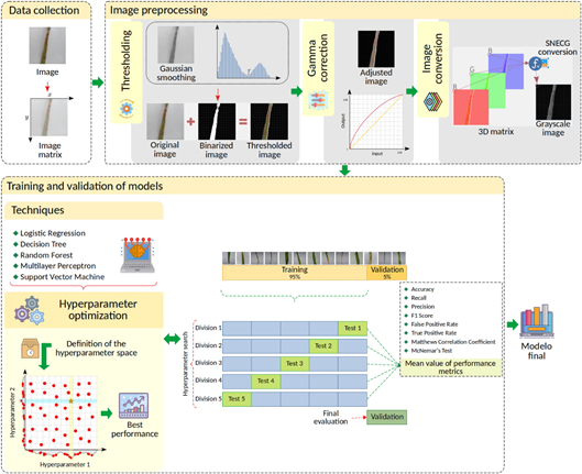
The flowchart depicted in Figure 1 illustrates the methodological approach employed in the development of this study, delineated into three principal steps, as explained below.
2.1. Data collection
The dataset for this study comprised images collected from five types of rice diseases obtained from secondary sources (Mendeley, 2022; IPM, 2023; IRRI, 2023). The collected image dataset consisted of 1538 images in JPEG (joint photographic experts’ group) format, with an original resolution of 4160 pixels in length and 1952 pixels in width.
The dataset included images of five major rice diseases: sheath blight (28.48%), rice blast (25.75%), leaf scald (18.60%), rice tungro (15.47%), and brown spot (11.70%). These images were systematically organized into separate folders based on the disease type. The labels for each class were generated using the folder structure, ensuring that all images within the same folder were assigned the same class label. Additionally, to streamline computational efficiency during model development, the images were resized to a resolution of 128 × 128 pixels.
2.2. Image preprocessing
To capture rice disease-specific characteristics, various image processing methods such as thresholding, gamma correction, and conversion to grayscale were applied, as illustrated in Figure 1.
Thresholding
A highly popular image segmentation technique is thresholding, which involves separating the foreground from the background of the image by creating binary images (Nixon & Aguado, 2019; Rajinikanth et al., 2020).
Image thresholding involves selecting a threshold T such that any pixel (x, y) satisfying f(x, y) > T can be termed an object pixel (Gonzales & Wintz, 2017). Among advanced thresholding techniques is optimal thresholding with Otsu’s method, which aims to find an optimal value, T, for separating the object from the background by employing a generalized grayscale histogram, where the number of pixels at each gray level is divided by the total number of pixels in the image (Nixon & Aguado, 2019; Gonzales & Wintz, 2017). Gaussian smoothing was employed to remove noise from the images (Gonzales & Wintz, 2017).
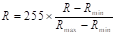
In the thresholding process, the probability distribution for the L gray levels of an image with dimensions M × N is provided by the mathematical formula in Equation 1:
 ()1
()1
where the gray level  ranges from 0 to 255,
  represents the number of pixels in the image with gray level , and MN = n0 + n1 + … + nL-1 denotes the total number of pixels. The threshold T = k (gray level) lies within the intensity range 0 < k < L - 1, dividing the image into classes c1 = [0, k] and c2 = [k + 1, L - 1]. Thus, given the threshold k, the probability of a gray level being classified into classes c1 or c2 is provided in Equations 2 and 3.
 ()2
()2
 ()3
()3
where P 1 (k) is the probability of class c 1 and P 2 (k) is the probability of class c 2 .
The average of gray levels for classes c 1 and c 2 is calculated as shown in Equations 4 and5 . Furthermore, the global mean of gray levels is calculated by Equation 6:
 ()4
()4
 ()5
()5
 )6
)6
where it must hold that P 1 (k) m 1 (k) + P 2 (k) m 2 (k) = m G and P 1 (k) + P 2 (k) = 1.
Thus, the global variance of the gray level across all image pixels is computed by  (Equation 7), while the between-class variance is calculated by
  (Equation 8). These variance measures are then used to calculate
  (Equation 9), which facilitates the evaluation of the effectiveness of the chosen threshold in separating the image components.
 ()
()
 (8)
(8)
 ()
()where the values of  are within the range
  . In this way, the optimal threshold T = k* must satisfy Equation 10:
 ()
()where  maximizes the between-class variance (Nixon & Aguado, 2019; Gonzales & Wintz, 2017).
Gamma correction
Gamma correction () adjusts the variations in luminance levels between individual pixels in an image, thereby enhancing visual appearance and highlighting specific features (Gonzales & Wintz, 2017). Thus, gamma correction in an image is calculated using the Equation 11:
 ()
()where s allows for a non-linear transformation of the color levels in the RGB (red, green, blue) channels, and the variables c and are positive constants (Nixon & Aguado, 2019).
Conversion to grayscale
Considering that an image is commonly represented in the RGB bands (Rafael et al., 2020; Gonzalez & Woods, 2018), the adjusted color images were simplified for processing through conversion to grayscale.
A simple and popular method is linear projection f(x) GS = α R × R + α G × G + α B × B, where the values of α R , α G , α B are non-negative and satisfy the constraint α R + α G + α B = 1 (Kanan & Cottrell, 2012; Gonzalez & Woods, 2018). The simplest method for converting images to grayscale is the average method, where the coefficient values correspond to one-third of the original values of the RGB channels (Ma et al., 2015).
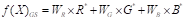
In this study, the SNECG method was utilized, which is based on the pixel neighborhood approach and is distinguished by its adaptive characteristics that enhance the brightness, contrast, and details of the images (Lim % Isa, 2011). The SNECG method is obtained through the formula presented in Equation 12:
 ()12
()12
where the coefficients W R , W G , and W B are estimated by averaging the coefficients T R , T G , and T B , which are obtained by summing the intensity levels of each RGB channel, as presented in Equations 13 and14:
 , and ()13
 , and ()14
The modified values of the coefficients R * , G * , and B * determine the extended values (Lim and Isa, 2011), which are calculated using the minimum and maximum values of the RGB channels, as presented in Equations 15 -17.
 , and ()15
 , and ()16
 , and ()17
2.3. Training and validation of models
In addition to image processing, this study was based on applying ML techniques due to their ability to identify complex patterns in high-dimensional datasets (Marsland, 2015; Alpaydin, 2021). ML is a subfield of artificial intelligence that uses computational and statistical techniques to create mathematical models that can recognize specific features in images (Jordan & Mitchell, 2015). Supervised ML classification techniques such as LR, DT, RF, Multilayer Perceptron (MLP), and SVM were used in this work. On the other hand, the optimal combination of hyperparameters for each model was obtained using the Random Search method.
The image dataset was divided into 95% for model training using the 5-fold cross-validation method, with its optimal hyperparameter configuration obtained via random search optimization. On the other hand, due to the class imbalance in the collected dataset, the oversampling technique was employed in each subdivision. This was done to mitigate the inherent bias in the unbalanced data (Rahman et al., 2015). The remaining 5% of images were utilized for model validation, as illustrated in Figure 1.
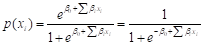
Logistic Regression
A classic statistical technique that fits an "S"-shaped curve, akin to linear regression, is utilized. This fitted curve is employed to compute the probability that the output y predicted by the model belongs to one of the k classes (Alpaydin, 2021). The logistic function for models aimed at calculating the probability of two classes is presented in Equation 18:
 ()18
()18
Where β 0 and β 1 are the parameters or coefficients of the model, which are calculated using the maximum likelihood method, and x i are the input variables (Alpaydin, 2021).
Decision Trees
The DT technique enables the construction of predictive models through a sequence of binary splits of the training dataset, structured with nodes and leaves. Specifically, in the context of classification trees, their construction involves an iterative process that begins with selecting the most significant feature from the dataset to form the root node (Alpaydin, 2021). Based on the root node, internal binary subdivisions occur, leading to the creation of internal nodes (t) until reaching the model’s leaves, where predictions are made (Marsland, 2015). These data subdivisions must satisfy , continuing until a reduction in error is achieved at each leaf node (Alpaydin, 2021).
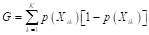
The leaves are also known as predictors d(x), and their prediction performance can be evaluated using the Gini index, a measure of homogeneity aimed at reducing data impurities from the root node to the leaf nodes (Alpaydin, 2021; Marsland, 2015). The Gini index represents a measure of total variance among K (k = 1, 2, …, K) classes (Gareth et al., 2013; Alpaydin, 2021; Marsland, 2015) and is calculated as shown in Equation 19:
 ()19
()19
where denotes the probability that a proportion of training data in node t belongs to class k (Gareth et al., 2013). A small value of G indicates that predictor d(x)
t
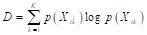
consists of data from one class (Gareth et al., 2013; Alpaydin, 2021). Another method to evaluate the constructed tree’s performance is by assessing the quality of data split using entropy calculation (Alpaydin, 2021), shown in Equation 20:
 ()20
()20
Like the Gini index, the entropy value D will be small if  is close to zero or one, indicating a high purity split (Gareth et al., 2013). Furthermore, the classification error rate, depicted in Equation 21, can be utilized to evaluate the accuracy of the final model, post-pruning using either entropy or the Gini index.
 ()21
()21
Multilayer Perceptron
The MLP models the relationship between input signals (input variables) and the output signal (target variable). Its basic structure consists of three main layers: the input layer, one or more hidden layers, and the output layer (Alpaydin, 2021).
The neurons in the input layer of the model receive the values to be processed, which flow through several hidden layers, considered the main computational drive. The output layer then performs the prediction or classification based on the information from the input layer (Khan et al., 2022). The interconnected layers of the neural network use the backpropagation technique to enhance prediction accuracy. The gradient is calculated using the error function with the neuron weights in this process. Additionally, each neuron in the model employs a nonlinear activation function (Alpaydin, 2021).
The output of each neuron in the MLP specifically depends on the preceding neurons and the network weights, which can be represented by Equation 22:
 ()22
()22
where  is the activation function, making its outputs known as activations, x
i
are the input variables, w
ij
are the synaptic weights, and is the bias (Alpaydin, 2021; Khan et al., 2022).
is the activation function, making its outputs known as activations, x
i
are the input variables, w
ij
are the synaptic weights, and is the bias (Alpaydin, 2021; Khan et al., 2022).
Random Forest
The RF technique is an extension of DT and is also known as one of the ensemble methods (Sheykhmousa et al., 2020; Gareth et al., 2013). This technique is characterized by its internal structure, which consists of a collection of classification models using DT, where each model is trained on a random subset of data (Sheykhmousa et al., 2020; Marsland, 2015). Each internal tree generated results in a class, this outcome is the class with the highest frequency (Belgiu & Drăguţ, 2016; Gareth et al., 2013).
In the RF, the L classification trees (f 1 (x), f 2 (x), …, f L (x)) trained are used to predict the final class f(x) (Belgiu & Drăguţ, 2016; Sheykhmousa et al., 2020). Specifically, f(x) is obtained through majority voting among the L classifiers (Belgiu & Drăguţ, 2016; Alpaydin, 2021).
Support Vector Machines
The SVM is noted for its efficiency with high-dimensional data, even when the number of dimensions exceeds the number of instances in the dataset (Marsland, 2015). This technique maps the input data into a higher-dimensional nonlinear feature space to find a hyperplane that maximizes the margin between classes by minimizing the distance between them (Islam et al., 2017; Sheykhmousa et al., 2020).
For constructing binary models, the classifier is obtained by solving a regularization problem that maximizes the margin between classes through the minimization of the associated objective function, as depicted in Equation 23 and24:
 ()
()subject to:
 ()
()where x
i
and y
i
denote the training data and labels, f(x) represents the classifier, C is a constant representing the regularization factor, and  are slack variables (Islam et al., 2017).
Evaluation and validation metrics
Evaluating and validating predictive models is crucial, as it helps measure the accuracy and overall performance of the models by assessing their error rates and efficiency. The cross-validation technique enables the evaluation of a model’s robustness by preventing overfitting and helping to estimate its performance in practical applications (Marsland, 2015; Alpaydin, 2021). In its application, the training dataset is randomly divided into k equally sized subsets (5-fold).
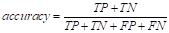
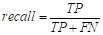
In this way, although there are various evaluation metrics available, no single standard metric has been established (Rodriguez et al., 2022). The formulas for the evaluation metrics adopted, based on the confusion matrix, are presented below in Equations 25 to30.
 ()
()
 ()
()
 ()27
()27
 ()28
()28
 ()29
()29
 ()30
()30
The Matthews correlation coefficient (MCC) was used to measure the quality of the classifications generated by the models (Zhu, 2020). The MCC is calculated as depicted in Equation 31.
 ()31
()31
The MCC value varies between {+1, -1}, with values close to +1 indicating perfect classification and those near -1 indicating perfect misclassification. Conversely, a value of 0 indicates random prediction, signifying the model’s inability to predict (Chicco, 2020).
Additionally, the McNemar test was utilized to validate the selection of the best final model by comparing and analyzing the frequency of errors or successes of each one. Hence, the comparison of models is grounded on the null hypothesis that both models possess the same error rate (H 0 : error M1 = error M2 ). The McNemar statistic (X 2 ) is calculated according to Equation 32.
 ()32
()32
The null hypothesis is rejected at a significance level of α if the value of X 2 is greater than X α,1 (Alpaydin, 2021).
3. Results and discussion
The optimal threshold values of the analyzed images per class showed a close variation within their value ranges. Figure 2 (A-B) illustrates the distribution of the optimal threshold values obtained for each image per class.
For the brown spot class, the threshold value k * varied between 103 and 149. For the leaf scald class, the range was between 105 and 147, while for rice blast, it ranged between 104 and 152. In the case of rice tungro, the threshold spanned from 105 to 149, and for the sheath blight class, it varied between 102 and 149 (Figure 2). Additionally, a gamma value of γ = 0.65 was utilized in the gamma correction method. Figure 2 (C) displays the curve of color levels of individual pixels corrected with the gamma value considered, resulting in brightness adjust ment of the dataset images. Improving the visual appearance of the images through thresholding and gamma correction methods emphasized specific characteristics of rice leaves, such as the lesions caused by the evaluated diseases.
The application of the SNECG method was chosen because, unlike the average method, SNECG demonstrated superior performance in the conversion of grayscale images, effectively capturing the inherent characteristics related to the color of each lesion associated with several types of diseases (Figure 3A).
The SNECG method enabled a more detailed capture of the brightness and characteristics of each color image during the conversion to grayscale, as shown in Figure 3 (B).
Next, the Table 1 presents the labels and the number of images per class for the training and validation processes.
Table 1 Dataset division for training and validation
| Class | Label | Training | Validation |
|---|---|---|---|
| Leaf scald | 0 | 271 | 15 |
| Rice blast | 1 | 375 | 21 |
| Brown spot | 2 | 173 | 7 |
| Sheath blight | 3 | 413 | 25 |
| Rice tungro | 4 | 229 | 9 |
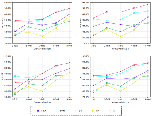
Among the training outcomes, each model exhibited varying performance based on the results of 5-fold cross-validation. Figure 4 presents the performance metrics, including accuracy, recall, precision, and F1-score.
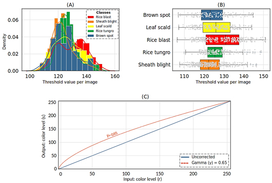
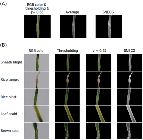
Figure 3 (A) Color-processed images and grayscale images produced using the average method and the SNECG method, along with (B) original and processed images using thresholding, gamma correction, and the SNECG method for each type of disease.
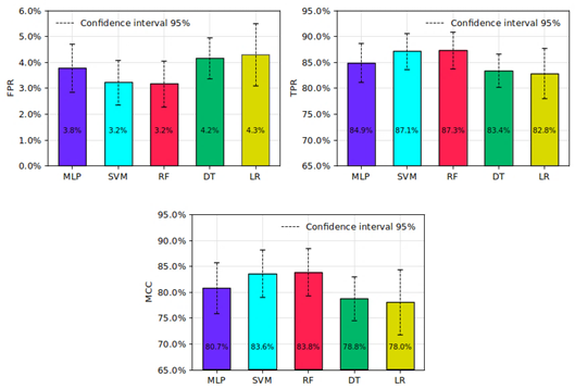
The performance analysis of the models trained using 5-fold cross-validation showed that all tested techniques achieved metrics above 78%, which can be considered acceptable. Figure 5 illustrates the mean values for the evaluation metrics FPR, TPR, and MCC, along with their corresponding confi dence intervals (95% CI) at a 5% significance level.
Upon inspection of the model training results (Figures 4 and5), it was observed that models generated using SVM and RF techniques achieved the highest number of correctly classified images. To facilitate the comparison of error metric results for each evaluated technique, Table 2 presents the mean values of the evaluation metrics obtained during model training.
As observed in Table 2, for the metrics of accuracy, precision, recall, F1-score, and TPR, all tested techniques exceeded 82.29%, while the FPR metric presented values below 4.30%. The results indicated that the models that used MLP, DT, and LR exhibited the lowest values in the evaluated performance metrics. Concerning the model trained with the LR technique, it was observed that it presented values similar to those obtained by Feng et al. (2020).
Additionally, the models trained with RF and SVM techniques achieved the best error metric values, with very close values to each other compared to models trained with other techniques (Table 2).
The MCC was used to measure the quality of the predictions of each trained model. It was found that all tested models obtained a mean MCC value above 78.05%. The MCC results demonstrated that models using RF (83.84%, with CI95%: 88.41 - 79.28) and SVM (83.58%, with CI95%: 88.14 - 79.02) showed the best prediction performance compared to the models using MLP (80.74%, with CI95%: 85.67 - 75.82), DT (78.76%, with CI95%: 82.95 - 74.57), and LR (78.05%, with CI95%: 84.36 - 71.74).
Based on the results obtained during the cross-validation training stage, the models using RF and SVM were retrained with the remaining 95% of the dataset to validate and select the final model. Table 3 presents the optimal hyperparameters for each model trained with each final ML technique.

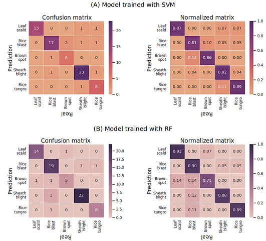
Considering that model validation was conducted using 5% (77) of the images, Figure 6 (A) presents the confusion matrix of classifications made with the SVM model, demonstrating that the model correctly classified 87.01% of the images. Figure 6 (B) presents the confusion matrix for the RF model validation, demonstrating that the model developed using this technique correctly classified 88.31% of the images. This technique exhibited behavior closely resembling the results obtained with SVM.
Table 3 Hyperparameters of the best ML models
| Model | Hyperparameter | Description | Parameter |
|---|---|---|---|
| RF | n_estimators | Number of classification trees. | 128 |
| max_features | Maximum number of features used to split a node. | sqrt | |
| criterion | Function to measure the quality of the split. | gini | |
| min_samples_split | Minimum number of features in a node before splitting. | 2 | |
| min_samples_leaf | Minimum number of features in a leaf node. | 1 | |
| bootstrap | Sampling method for constructing the trees. | False | |
| SVM | C | Regularization parameter. | 125 |
| decision_function | Decision function. | ovr | |
| max_iter | Maximum iteration limit. | -1 | |
| kernel | Kernel function. | rbf | |
| gamma | Kernel coefficient. | scale |
The McNemar test results (Table 4) indicated no significant differences between the errors of the models. These findings suggested the need for a more detailed evaluation to select the final model.
Table 4 Results of the McNemar test in the validation process
| Models | X2 | X0,05,1 | Description |
|---|---|---|---|
| RF | 0.001 | 3.84 | Accept H 0 |
| SVM |
The metrics results of both models were remarkably similar; however, the RF model exhibited higher precision and accuracy exceeding 88%, which outper-formed the SVM technique (Table 5). Additionally, the Matthews correlation coefficient indicated that the RF model achieved better performance, slightly surpass-sing the SVM model with a coefficient close to 85%.
Table 5 Evaluation metrics results with validation images
| Models | SVM | RF |
|---|---|---|
| Accuracy | 87.01% | 88.31% |
| Precision | 86.84% | 86.43% |
| Recall | 85.13% | 88.07% |
| F1 | 85.61% | 87.05% |
| TPR | 87.01% | 88.31% |
| FPR | 3.25% | 2.92% |
| MCC | 83.13% | 84.74% |
Contrasting these results with some observed in the literature, it is noteworthy that the studies by Tian et al. (2021), Azim et al. (2021), and Feng et al. (2020) developed models using ML techniques that achieved lower accuracy than the SVM and RF techniques used in this study.
Moreover, it is important to note that one of the main differences between those studies and this re search is that their models were developed to clas sify only one to three types of rice diseases, while this work evaluated five types of diseases. Table 6 presents the types of diseases considered by various authors for the development of classification models. ML techniques have been widely applied to the identification of various rice diseases. Among these, the most frequently studied include brown spot, blast, bacterial blight, and leaf smut (Lu et al., 2017; Feng et al., 2020; Sethy et al., 2020; Azim et al., 2021; Jiang et al., 2021; Elmitwally et al., 2022). However, when comparing the findings of these studies with the results of the present in vestigation, no prior research was identified that comprehensively evaluated the diseases sheath blight, tungro, blast, leaf scald, and brown spot in an integrated manner.
Table 6 Types of diseases analyzed in various published research
| Research | Rice diseases | ||||||||||||||
| (a) | (b) | (c) | (d) | (e) | (f) | (g) | (h) | (i) | (j) | (k) | (l) | (m) | (n) | (o) | |
| Lu et al. (2017) | ✓ | ✓ | ✓ | ✓ | ✓ | ✓ | ✓ | ✓ | ✓ | ✓ | |||||
| Sethy et al. (2020) | ✓ | ✓ | ✓ | ✓ | |||||||||||
| Jiang et al. (2021) | ✓ | ✓ | ✓ | ||||||||||||
| Tian et al. (2021) | ✓ | ||||||||||||||
| Azim et al. (2021) | ✓ | ✓ | ✓ | ||||||||||||
| Upadhyay y Kumar (2021) | ✓ | ✓ | |||||||||||||
| Feng et al. (2020) | ✓ | ✓ | ✓ | ||||||||||||
| Sharma et al. (2022) | ✓ | ✓ | ✓ | ✓ | |||||||||||
| Latif et al. (2022) | ✓ | ✓ | ✓ | ✓ | ✓ | ||||||||||
| Kumar y Kannan (2022) | ✓ | ✓ | ✓ | ||||||||||||
| Rallapalli y Saleem (2021) | ✓ | ✓ | ✓ | ✓ | ✓ | ||||||||||
| Elmitwally et al. (2022) | ✓ | ✓ | ✓ | ||||||||||||
| Akyol (2023) | ✓ | ✓ | ✓ | ||||||||||||
| Reddy et al. (2022) | ✓ | ✓ | ✓ |
NOTE. (a): Blast, (b): False smut, (c): Brown spot, (d): Bakanae, (e): Sheath blight, (f): Sheath rot, (g): Bacterial blight, (h): Bacterial sheath brown rot, (i): Seeding blight, (j): Bacterial wilt, (k): Tungro, (l): Leaf smut, (m): Leaf scald, (n): Narrow brown spot, (o): Hispa
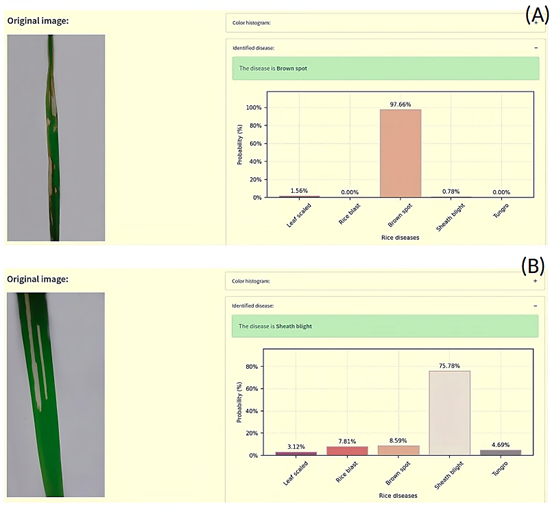
Finally, Figure 7 illustrates an interface developed by integrating the best model with RF to diagnose the type of disease present in the rice leaf. The developed interface allows for observing the classification result, in addition to the probability that the leaf presents the identified disease. In Figure 7 (A), the identification of brown spot disease with a 97.66% probability of ac curacy, and in Figure 7 (B), the identification of sheath blight disease with a 75.78% probability of accuracy.
4. Conclusions
Rice is one of the most widely consumed foods globally, and its production faces significant challenges due to the risk of infections from pests and diseases that can negatively impact efficiency and quality. This study applied various image processing methods, such as thresholding, gamma correction, and grayscale conversion using the SNECG method, to characterize disease lesions on rice leaves. Additionally, ML techniques were explored to develop a predictive model for the early detection of crop issues.
Five ML techniques were applied, including RF, LR, MLP, DT, and SVM, with cross-validation and random search for hyperparameter optimization. The results showed that all models correctly classified more than 80% of the images; however, the models with the best performance during training were the SVM and RF models. Validation of the top models indicated that the classifications made with the RF model were more accurate, making it the final selected model, with an accuracy exceeding 88%.
These results highlight that the integration of advanced image processing methods with ML techniques enables the development of highly efficient classification models and opens new possibilities for the precise detection of specific issues in rice crops, leading to a significant improvement in their pro duction.
Moreover, by facilitating more effective management of agricultural diseases, these emerging tools play a crucial role in strengthening food security through more informed and proactive agricultural practices. This approach with ML models can not only optimize the management of agricultural resources but also promote more responsible and effective practices in food production, thereby fostering a more robust and secure agricultural system for future generations.
Finally, for future research, the application and comparison of other ML techniques are recommended, as well as the integration of other types of diseases affecting rice crops, to develop a more robust tool.

