Problematic Situation

^{Ñaupas et al. (2014}) indicate that in daily life there are repetitive patterns, with certain different characteristics, and that the prediction of natural phenomena is more accurate than social phenomena:

Así por ejemplo, conociendo las leyes de Kepler, que explican los movimientos de traslación de los planetas, satélites, cometas y asteroides es posible calcular la ocurrencia de eclipses, mareas y acercamiento de cometas a la órbita de la Tierra. La predicción del tiempo, de inundaciones, terremotos, huracanas, erupciones volcánicas, la ocurrencia de mareas, o de pandemias son más confiables que las ocurrencias de revoluciones, conflictos sociales, golpes de estado, etc.[Thus, for example, knowing Kepler's laws, which explain the translational movements of planets, satellites, comets and asteroids, it is possible to calculate the occurrence of eclipses, tides and approach of comets to the Earth's orbit. The prediction of the weather, floods, earthquakes, hurricanes, volcanic eruptions and the occurrence of tides, or pandemics are more reliable than the occurrence of revolutions, social conflicts, coups d'état, etc.]. (section 2.4.2.¿Qué es la investigación natural?)

These phenomena, that originate crises, impact economies and finances in a negative way, which is why ^{Mira (2016}) considers the recurrent occurrence of financial crises. These crises have repeatedly affected the returns of the private pension system in Peru.

The International Labor Organization (ILO) established in 1933 the Convention on Old-Age Insurance, and in 1952 determined the guidelines for old-age benefits. In Peru the National Pension System (SNP), which is currently administered by the Pension Standardization Office (ONP) operated in the beginning. Between 1981 and 2014, as noted by ^{Ortiz, Durán-Valverde, Urban, Wodsak, and Yu (2019}), about 30 countries fully or partially privatized their mandatory public pensions, a fact that occurred in Peru in 1993. The Asociación de Administradoras de Fondo de Pensiones[3] (2018) defines the pension in the Peruvian private pension system (SPP) asel ingreso periódico que recibe el afiliado como consecuencia de un proceso previo de suavización de consumo, a través del ahorro a lo largo de su vida laboral en su cuenta de capitalización individual (CIC)[the periodic income received by the member as a consequence of a previous process of consumption smoothing, through savings throughout his working life in his individual capitalization account (CIC)] (p. 8) with the purpose of ensuring that the retired worker does not face economic difficulties.

AFPs are responsible for managing the contributions of each individual during his working life, that is, they invest their savings in order to obtain a return so that, once retired, the individual can enjoy their contributions and earnings with no need to depend on their family or the State. However, ^{Cruz-Saco et al. (2014}) pointed out that the pension system in Peru wasineficiente, tiene una baja probabilidad de incrementar apreciablemente la cobertura en los siguientes 36 años, y presenta, además, un conjunto de inequidades en la asignación de los beneficios previsionales[inefficient, has a low probability of appreciably increasing coverage in the next 36 years, and also presents a set of inequities in the allocation of pension benefits] (p. 2).

^{Flórez (2014}) also adds thatlos ahorros para la jubilación de millones de personas se encuentran expuestos, de manera intrínseca, al comportamiento favorable, así como adverso, de los mercados financieros[the retirement savings of millions of people are intrinsically exposed to the favorable and adverse behavior of financial markets] (p. 121). These situations are the cause of high volatility, especially when there is more negative news than positive, so an asymmetric behavior of the market, especially the equity market, is observed.

^{Ortiz et al. (2019}) argue thatLos trabajadores se convirtieron así en consumidores obligados del sector financiero, con lo que asumían individualmente todos los riesgos del mercado financiero sin contar con la suficiente información para tomar decisiones sensatas[Workers became forced consumers of the financial sector, thus individually assuming all the risks of the financial market without enough information to make reliable decisions] (p. 803). In other words, when the market is stable or when there is good news, returns will be positive. On the other hand, according to Yang et al. (as cited in ^{Gutiérrez et al., 2017}), financial crises have been characterized by the increase of risk and high volatility, which has negatively affected returns. In the case of the SPP, as a consequence of negative news, the high expectations the SPP initially generated were diluted as the years went by because it did not produce the expected results.

Carlos Palomino, in an interview with RTV San Marcos - UNMSM (2020), stated that the investments of AFPs go into stock-market mechanisms and not into tangible assets. These stock-market instruments are volatile due to economic shocks or cycles which, in turn, are a consequence of external variables, such as, for example, a pandemic.

It should be noted that in November 2006, the absorption of AFP Unión Vida by Prima AFP was authorized. In April 2013, AFP Horizonte was acquired by AFP Integra and Profuturo (50% each). AFP Habitat began operations in April 2013.

The type 2 fund began operations in December 2005. Its investments are distributed 55% in fixed income and 45% in equities, with a balanced profile aimed at workers aged 45 to 60. Figure 1 shows a slight upward trend with a sharp drop during the world crisis between 2007 and 2008; a slight drop in April 2011 and 2016 during the first electoral rounds, as well as between 2018 and 2019, which culminated with the dissolution of the Congress of the Republic of Peru; and a sharp decline in March 2020 as a result of COVID-19. This performance corresponds to the monthly average in soles of the daily quota values used for calculating the profitability of the AFPs of type 2 fund.

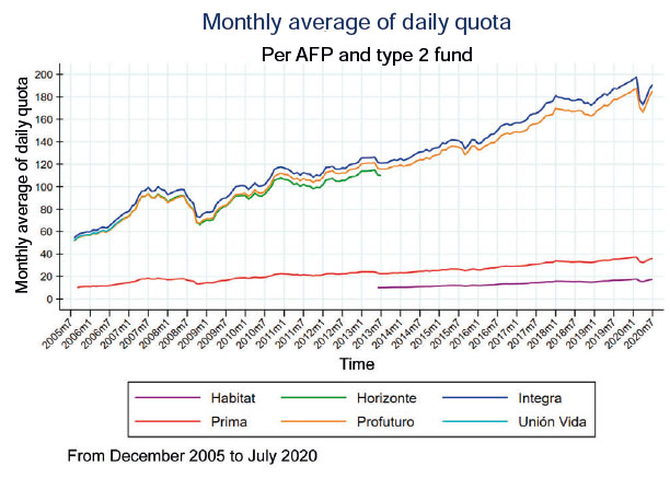
Source: Prepared by the author using Stata 16.

Figure 1 Monthly average of quota values for each AFP and type 2 fund. 

This work is very useful for workers between 45 and 60 years old, since their investments, managed by the AFPs, are affected by the economic and financial crises in the world. As these crises affect the returns of the Peruvian private pension system, the savings of workers are affected at the time of their retirement. Why did the response to recurrent financial risks adopted by the risk managers of AFPs not mitigate the loss of investment returns of workers? That is the big question asked by workers. Using the Box and Jenkins or ARIMA methodology, the behavior of the monthly average of the daily values of the type 2 fund for each AFP is described, as well as their forecast.

The objective of this research is to determine how to adequately model the monthly average of the quota values for each AFP of the type 2 fund with the Box and Jenkins methodology.

Moreover, this research specifically seeks to determine if the trend of the monthly average of the quota values for each AFP of the type 2 fund influences the unit root, if stationarity influences its mean and variance, and if there is correlation between the observed values and the forecast values.

General Hypothesis

The monthly average of the quota values for each AFP of the type 2 fund will be adequately modeled with the Box and Jenkins methodology.

Specific Hypotheses

Identification

In this part, it was verified, based on the unit root (UR) tests, whether the series of the four AFPs were stationary; in addition, it was verified that the series had memory or that they did not have white noise, since otherwise, they could not be forecast with the Box and Jenkins methodology. For this, the following substeps were performed: graphical analysis, statistics calculations, unit root tests and white noise tests.

Estimation

Based on the results of the correlograms, the order of the AR and MA were identified using maximum likelihood estimation and the trial and error method from the statistical significance of each estimated coefficient.

Diagnostic Checking

The unit circle was used to validate the stability of the model, to corroborate that the residuals and squared residuals are white noise, and finally to perform the constant variance test with the following substeps: validation of the unit circle, validation of the residuals, and validation of the squared residuals.

Forecasting

A static forecastt+1-that is, one period ahead-was performed to calculate the error statistics. Subsequently, a dynamic forecastt+kperiods was performed.

Identification

Graphical Analysis

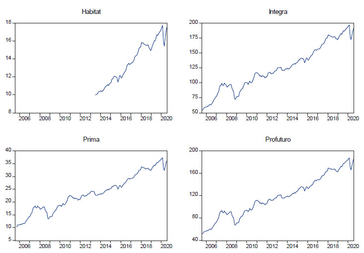
These are non-formal tests. ^{Court and Rengifo (2011}) argue that they help to determine the model and the order that best fit the data, since graphical methods and information criteria are used. Figure 2 shows the development of the monthly series of AFP Habitat, Integra, Prima and Profuturo, which show upward trends.

Source: Prepared by the author using Eviews 10

Figure 2 Behavior of the monthly average series of AFP Habitat, Integra, Prima and Profuturo by levels. 

Statitics Calculation

Figure 2 shows that the original series of AFP Profuturo has a trend, but, in the results of the model in Figure 3 (left side), it has a p-value of 4. 95%, that is, less than 5%, so the H₀(which states that the series has a UR) is rejected and, therefore, it is stationary; however, in the same Figure 3 (right side), it can be observed that the autocorrelation does not decay exponentially to corroborate that the original series is stationary; on the contrary, it decays linearly, which indicates that it is not stationary and must be differentiated.

Source: Prepared by the author using Eviews 10.

Figure 3 Statistics Calculation for AFP Profuturo. 

Figure 4 shows that the original series of AFP Habitat, Integra and Prima have at least one UR and, therefore, are not stationary. ^{Gujarati and Porter (2010}) point out that “Each set of time series data will therefore be for a particular episode. As a consequence, it is not possible to generalize it to other time periods”. For forecasting time series, non-stationary time series are not very useful, and to overcome this obstacle, the original series must be differentiated to make them stationary.

Source: Prepared by the author using Eviews 10.

Figure 4 Statistics Calculation for AFP Integra, Prima and Profuturo. 

Unit Root Tests

Dickey Fuller Augmented (DFA) tests, which according to ^{Bello (2018}) are the test most widely used, were performed on the original series of Habitat, Integra, Prima and Profuturo.

When performing the hypothesis tests to those series, the null hypotheses that suggested that the series have at least one UR were not rejected, therefore, the logarithmic differentiation of their original series was applied to make them stationary. Figure 5 shows the results of the models.

Source: Prepared by the author using Eviews 10.

Figure 5 Unit root tests. 

White Noise Tests

It was verified that the time series already differentiated had memory using correlograms and the Ljung Box (LB) statistic for small samples. Figure 6 shows the correlograms for Habitat, which showed that up to month seven there is no white noise and, from month eight, the impact on the current Habitat series is not significant. In the case of Integra, there is no white noise up to month fifteen. As for Prima, there is no white noise up to month thirteen. Finally, Profuturo has no white noise until month sixteen and, after this month, the impact is not significant in the result of the current series. In conclusion, the differentiated series of AFP Habitat, Integra, Prima and Profuturo are stationary and have no white noise and, therefore, can be forecast with the Box and Jenkins methodology.

Source: Prepared by the author using Eviews 10.

Figure 6 White noise tests. 

Estimation

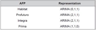
Based on the results of the correlograms, the order of the AR and MA were identified using maximum likelihood estimation, and the trial and error method, based on the statistical significance of each estimated coefficient. Using Eviews software, the best model was automatically selected by running iterations with combinations of the AR, MA and order of integration. In this case, 484 models were run for each AFP, and the model with the lowest Akaike Info Criterion (AIC) was chosen, as shown in Figure 7.

Source: Prepared by the author using Eviews 10.

Figure 7 Identification of the order of AR and MA. 

The representations of this model are shown in Table 1.

Table 1 Selection of ARIMA Models. 

Source: Prepared by the author.

Validation

Unit Circle Validation

The validation with the unit circle was performed and, as shown in Figure 8, it can be seen that the models are stationary in the autoregressive part for AFP Prima, Profuturo and Integra. It is also observed that the models of AFP Habitat, Profuturo and Integra are invertible in the moving average part. None of the roots of the four AFPs are outside the unit circle, and all their moduli are below 1, so it is concluded that they passed the unit circle validation tests.

Source: Prepared by the author using Eviews 10.

Figure 8 Unit circle validation. 

Validation of the residuals

Subsequently, the correlogram was performed to verify that the residuals had white noise. In Figure 9, it was verified that the behavior of the residuals of the four AFPs has white noise because their p-values are greater than 5% and, therefore, forecasting with the Box and Jenkins ARIMA models is possible.

Source: Prepared by the author using Eviews 10.

Figure 9 Validation of the residuals. 

Validation of the squared residuals

The squared residuals of the 4 AFPs also presented white noise, since all theirp-values are above 5%, as shown in Figure 10; if this had not been the case, it would have been necessary to perform an equation to the variable and then work with the conditional volatility models ARCH and GARCH.

Source: Prepared by the author using Eviews 10.

Figure 10 Validation of the squared residuals. 

Forecasting

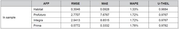
Curt and Rengifo (2011) argue thatPara determinar si un pronóstico es adecuado, se usan los estadísticos que (…) comparan los valores reales con aquellos que han sido pronosticados. (…) como los errores pueden ser positivos o negativos, (…) suma de ellos no sería de gran ayuda puesto que se cancelarían entre ellos. Es por eso que los índices trabajan ya sea con los errores al cuadrado o con el valor absoluto de los errores[To determine whether a forecast is adequate, statistics that (...) compare actual values with those that have been predicted are used. (...) as errors can be positive or negative, (...) to use addition with them would not be of great help since they would cancel each other. That is why the indices work either with squared errors or with the absolute value of the errors] (pp. 427-428); so static forecasts of the monthly average of the quota values of each of the four AFPs are performed in order to take into account the following error statistics:RMSE(Root Mean Square Error),MAE(Mean Absolute Error),MAPE(Mean Absolute Percentage Error) andU-THEIL(Theil’s Inequality Coefficient), which are contained in Table 2.

Table 2 Forecast Errors with ARIMA. 

Source: Prepared by the author.

Table 2 shows that AFP Habitat has the lowest forecast error with ARIMA, since its RMSE, on average, deviates by 0.2796 units and in percentage terms or MAPE, the deviation is 1.20%. AFP Integra has the highest RMSE with respect to the other three AFPs, with a deviation of 2.8076 units. In percentage terms, AFP Prima has the highest deviation with 1.66%.

The forecasts with ARIMA were compared with the double exponential smoothing techniques contained in Table 3, which were automatically selected out of eight techniques by the Risk Simulator software for having the lowest error statistics; these techniques are contained in Table 3 and it is observed that ARIMA has lower forecast errors than double exponential smoothing.

Table 3 Forecast Errors with Double Exponential Smoothing Techniques. 

Source: Prepared by the author.

Hypothesis Testing

Specific hypothesis 1: The trend of the monthly average of the quota values for each AFP of the type 2 fund directly influences the unit root.

Table 4 shows that the original series of AFP Profuturo does not show a trend and itsp-value is equal to 4.95%, less than 5%, so the H₀(which states that the series has a UR) is rejected and, therefore, the series is stationary. Table 4 also shows that thep-values of Habitat, Integra and Prima are above 5%, so the H₀s are not rejected since they have at least one UR and are not stationary.

Table 4 Unit Root Hypothesis Tests for AFPs Habitat, Profuturo, Integra and Prima. 

Source: Prepared by the author.

Specific hypothesis 3: Stationarity directly influences the variance of the return of the monthly average of the quota values for each AFP of the type 2 fund.

A differentiation was made for each AFP, and the results of the hypothesis tests contained in Table 5 indicate that their p-values are less than 5% and, therefore, the null hypotheses are rejected. The differentiated series for each AFP has no unit root and is therefore stationary with constant mean.

Table 5 Hypothesis Test for the Mean of AFPs Habitat, Integra, Prima and Profuturo. 

Source: Prepared by the author.

Specific hypothesis 3: Stationarity directly influences the variance of the return of the monthly average of the quota values for each AFP of the type 2 fund.

It is verified that the differentiated series have no memory using the Ljung Box (LB) statistic for small samples. The joint tests for the squared residuals of the four AFPs present white noise, since all theirp-values are above 5%, as shown in Table 6.

Table 6 Hypothesis Test for the Variance of AFPs Habitat, Integra, Prima and Profuturo. 

Source: Prepared by the author.

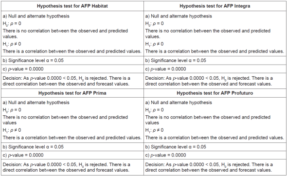
Specific hypothesis 4: There is a correlation between the observed values of the monthly average of the quota values for each AFP of the type 2 fund and the predicted values.

Table 7 shows that the results of the correlation coefficients of the observed values of the monthly average of the quota values for each AFP of the type 2 fund and the predicted values correspond to strong positive correlations; the table also contains theirp-values.

Table 7 Results of Pearson's correlation coefficient. 

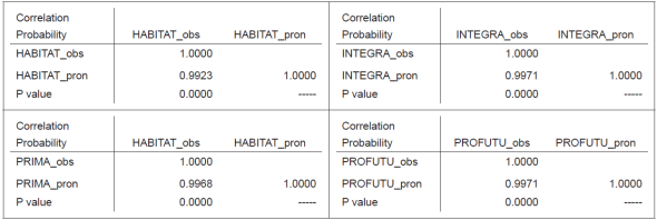
Source: Prepared by the author.

Note: the results are presented as reported by the software.

In the hypothesis tests contained in Table 8, it is observed that thep-values of each AFP are below 5%, therefore, in addition to the strong and direct correlation between the observed and predicted values, these can be corroborated with the results of the error statistics contained in Table 3.

Table 8 Hypothesis tests for Pearson’s correlation of AFP Habitat, Integra, Prima and Profuturo. 

Source: Prepared by the author.