http://dx.doi.org/10.19083/ridu.10.495

ARTÍCULO METODOLÓGICO

Computer Programs for Comparing Dependent Correlations

Programas informáticos para comparación de correlaciones en muestras dependientes

Programas de informática para comparações entre correlações: amostras dependentes

 

N. Clayton Silver*, César Merino-Soto**

*Department of Psychology, University of Nevada, Las Vegas, USA

** Instituto de Investigación de Psicología, Universidad de San Martín de Porres, Lima, Perú

---

ABSTRACT

There are a variety of techniques for testing the differences between dependent correlations that are not available using the standard statistical software packages. Examples of these techniques for examining different hypotheses within the dependent correlational realm are presented along with the output and interpretation from easily attainable, userfriendly, interactive software.

Keywords: Computer Software, Statistics, Correlation, Dependent Correlations

---

RESUMEN

Existe una variedad de técnicas para probar las diferencias entre correlaciones dependientes que no están disponibles en los programas estadísticos estándar para el investigador. Se presentan ejemplos de estas técnicas para evaluar diferentes hipótesis dentro del contexto de correlaciones en muestras dependientes, junto con programas informáticos interactivos, de fácil uso y libre distribución.

Palabras clave: software, estadística, correlación, correlaciones dependientes

---

RESUMO

Existe uma variedade de técnicas para provar as diferencias entre correlações dependentes que não estão disponíveis nos programas estatísticos familiares para o investigador. Apresentam-se exemplos destas técnicas para avaliar diferentes hipóteses dentro do contexto de correlações em amostras dependentes, junto com programas de informáticas interativos, amigáveis e livre distribuição.

Palavras-chave: software, estatística, correlações, correlações dependentes

---

There are times when researchers are interested in determining if two correlations within the same sample differ from each other. Indeed, there are various techniques for examining hypotheses along these lines. However, tests for comparing correlations have been, at best, perfunctorily addressed in statistics textbooks. Moreover, because these techniques are not available using the standard statistical software packages, researchers have either been ignorant of these techniques or not implemented them based on mathematical complexity. Therefore, the purpose of this piece is to familiarize the reader with a number of these techniques and to describe user-friendly software that will perform these procedures.

COMPARING DEPENDENT CORRELATIONS – ONE ELEMENT IN COMMON

Suppose that a researcher is interested in determining whether the correlation between job satisfaction and salary is higher than the correlation between job satisfaction and supervisor satisfaction among a group of high school teachers. Because these correlation coefficients are obtained from the same sample, they would be considered dependent. Specifically, this is a test of dependent correlations with one element in common (i.e., job satisfaction), with the null hypothesis being ρ₁₂ = ρ₁₃. This hypothesis test has been seen often in the literature. For example, Grygiel, Humenny, Rebisz, Świtaj, and Sikorska (2011) examined the differences in the correlations between the Polish Version of the UCLA Loneliness Scale scores with the De Jong Gierveld Loneliness Scale scores and the UCLA Loneliness Scale scores. Moreover, Yoo, Steger, and Lee (2010) examined the correlation between subtle racism and treatment/aggression with blatant racism and treatment/aggression. Finally, Schroeder (2014) examined the correlation between younger adults’ selfpaced reading and sentence span with timed reading and sentence span.

In order to test this hypothesis, numerous procedures have been proposed and examined via simulation methods. Formulas for these procedures can be found in Hittner, May, and Silver (2003). For example, Neill and Dunn (1975) found that Williams’s (1959) modification of Hotelling’s (1940) t performed best in both Type I error rate and power, even when the sampling distribution of r was skewed. Likewise, Dunn and Clark’s (1969) z test also controlled Type I error rate effectively while maintaining adequate power. Hotelling’s t was more powerful than both tests, however, the Type I error was inflated (Neill & Dunn, 1975; Steiger, 1980). Similar to the results of Neill and Dunn (1975), Boyer, Palachek, and Schucany (1983) also found that Williams’s t showed reasonable control of Type I error and exhibited good power. However, they also found that the Type I error rates and power of Williams’s t were less than adequate when they used the lognormal distribution, which is highly skewed.

In an examination of Williams’s t, Hotelling’s t, Olkin’s (1967) z, and Meng, Rosenthal, and Rubin’s (1992) z, May and Hittner (1997) found that the z tests showed reasonable control of Type I error while exhibiting good power. The t tests, on the other hand, exhibited greater power based on an inflated Type I error. However, the May and Hittner (1997) simulation was based on a Williams t which was published by Hendrickson, Stanley, and Hills (1970). This formula was different than the Williams’s t reported by other researchers (e.g., Neill & Dunn, 1975; Steiger, 1980).

In a more comprehensive study, Hittner et al.(2003), examined eight test statistics (Hotelling’s t, Williams’s "standard" t. Williams’s t (Hendrickson et al., 1970), Olkin’s z, Meng, Rosenthal, and Rubin’s z, Dunn and Clark’s z , Steiger’s (1980) modification of Dunn and Clark’s z using an arithmetic average correlation of ρ₁₂ and ρ₁₃ and Steiger’s (1980) modification of Dunn and Clark’s z using a backtransformed average z of ρ₁₂ and ρ₁₃). The backtransformed average z approach was chosen based on the premise that it has less bias and greater accuracy for estimating the population correlation coefficient than the arithmetic average, particularly when ρ was .50 and above (Silver & Dunlap, 1987). Under a normal distribution and a sample size of 20, their results indicated that Type I error rates for Hotelling’s t and the Hendrickson et al. (1970) version of Williams’s t were high when the predictor-criterion correlations (i.e. ρ₁₂ and ρ₁₃) were high (e.g., .70) and the predictor intercorrelation (ρ₂₃) was low. Olkin’s z had an inflated Type I error rate when the predictor-criterion correlations were low to moderate (.10 or .40). Williams’s "standard" t, Dunn and Clark’s z, Meng, Rosenthal, and Rubin’s z, and the two Steiger modification tests exhibited reasonable control of Type I error and good power. Although it appears that the Meng, Rosenthal, and Rubin z has a little better control of Type I error (i.e., less deviation from the nominal level) than the other tests.

However, under a uniform distribution, these five tests were conservative when the predictor-criterion correlations and the predictor-intercorrelation were high (e.g., .70). Under an exponential distribution, these tests had inflated Type I error rates for moderate to high predictor-criterion correlations. The liberalness increased as the predictor-criterion correlation increased. However, even with sample sizes of 300, these tests still had problematic Type I error rates. Of interest, regardless of distribution, as the predictor-intercorrelation increased, power did as well for all tests. Nevertheless, because of these Type I error deficits, there appears to be no optimal significance test.

Wilcox and Tian (2008) suggested a couple of different methods (D₁ and D₂) for combating these problems. Method D₁ may be a bit conservative, thereby lowering power, whereas Method D₂, using simulations to determine the critical value, may have more satisfactory characteristics. Their functions are written in R or S-Plus and would still need a main routine to work.

For the basic researcher, with limited to no computer programming experience, this can be problematic. Nevertheless, Silver, Hittner, and May (2006) wrote a user-friendly, interactive program (DEPCOR) for computing the aforementioned five tests. In this Windows program, the user is asked for the sample size, labels for each correlation, and the values of r₁₂, r₁₃, and r₂₃ for each group.

Let us suppose that for 100 high school teachers, the correlation between job satisfaction and salary was .60 and for job satisfaction and supervisor satisfaction it was .30. Moreover, the correlation between salary and supervisor satisfaction was .40. Figure 1 illustrates the output from DEPCOR.

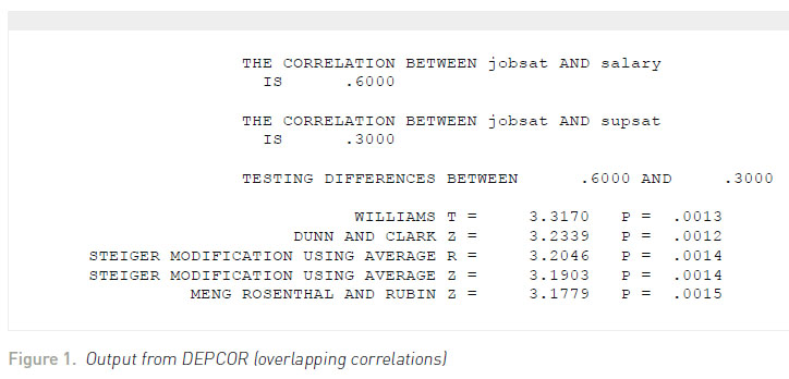
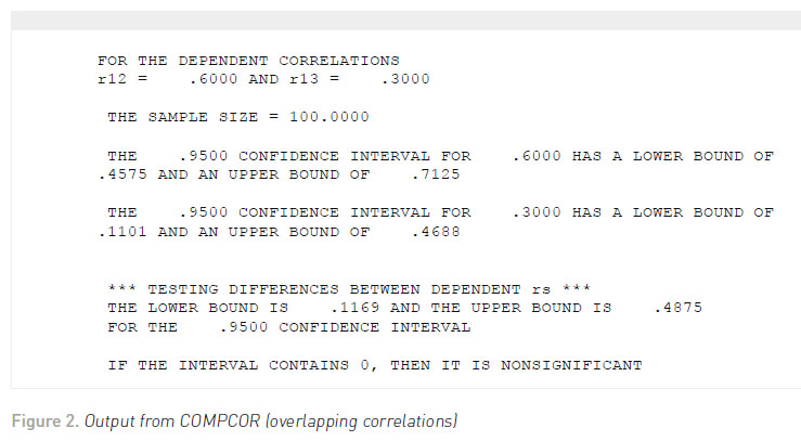
Regardless of the test, we would conclude that there is a significantly higher correlation between job satisfaction and salary than between job satisfaction and supervisor satisfaction. Zou (2007) suggested that confidence intervals could also be used for examining differences between dependent correlations with one element in common. Zou’s (2007) simulation indicated that this approach had better Type I error properties than the standard significance tests. Therefore, the interactive, user-friendly program COMPCOR (Silver, Ullman, & Picker, 2015) queries the user for the dependent correlations, sample sizes for each correlation, and percentage around which the confidence interval falls (e.g., .95). The output from COMPCOR is contained in Figure 2 . The confidence interval limits fall around .1169 and .4875. Because the confidence interval does not fall around zero, then a statistically significant result (p <.05) would be obtained.

COMPARING DEPENDENT CORRELATIONS – NO ELEMENTS IN COMMON

Aside from having overlapping correlations, there is an instance when one could have dependent correlations with nonoverlapping correlations or no elements in common. For example, suppose that one is interested in examining the correlation between job satisfaction and salary among high school teachers. This correlation is computed at the beginning of the academic year. However, suppose in the middle of the academic year, a 6% salary raise is given across the board. The correlation is then determined at the end of the academic year. In this case, the null hypothesis tested would be ρ₁₂ = ρ₃₄; that is, there is no statistically significant difference between the population correlation coefficients of job satisfaction and salary at the beginning and end of the school year. Examples from the literature include determining if the test-retest reliabilities of two different trauma measures are different (Wilker et al., 2015) and examining the difference in the correlations between auditory digits forward and backward with visual digits forward and backward (Kemtes & Allen, 2008).

There are four procedures examined by Silver, Hittner, and May (2004) for testing this hypothesis. They performed a Monte Carlo simulation evaluating the Pearson-Filon (1898), Dunn and Clark (1969), and the Steiger (1980) modification of Dunn and Clark’s z using an arithmetic average correlation of ρ₁₂ and ρ₃₄ and Steiger’s (1980) modification of Dunn and Clark’s z using a backtransformed average z of ρ₁₂ and ρ₃₄. They found that given a normal distribution, the Pearson-Filon (1898) approach exhibited high Type I error rates when ρ₁₂ and ρ₃₄ were low or moderate (.10 or .30). The other three tests exhibited more conservative Type I error rates when ρ₁₂ and ρ₃₄ were low or moderate (.10 or .30). Of course, all tests became more nominal as the sample size increased. However, even with a sample size of 100, the other three tests still had conservative Type I error rates when ρ₁₂ and ρ₃₄ were low (.10). Given a uniform distribution, the Pearson-Filon (1898) test exhibited the same behavior, whereas the other three tests were fairly conservative across the board. Finally, under an exponential distribution, the Pearson-Filon (1898) test was liberal under all conditions, whereas the other three tests had liberal Type I error rates when ρ₁₂ and ρ₃₄ were high (.70), but conservative when ρ₁₂ and ρ₃₄ were low or moderate (.10 or .30). The power differential among these three tests was negligible under all conditions. Therefore, even though these tests are not optimal, they appear to be the best statistical significance tests at this time. The program DEPCOR also performs these three tests as well. In this case, the user is asked for the sample size, labels for each correlation, and the values of r₁₂, r₁₃, r_14, r₂₃, r₂₄, and r₃₄ for each group.

Let us suppose that the correlation between job satisfaction and salary at the beginning of the year was .30 and at the end of the year it was .60 for the 100 high school teachers. Moreover, the correlation between job satisfaction at time 1 and time 2 is .40; the correlation between job satisfaction at time 1 and salary at time 2 = .20; the correlation between job satisfaction at time 2 and salary at time 1 = .25; and the correlation between salary at time 1 and salary at time 2 = .50. The output from DEPCOR is shown in Figure 3 .

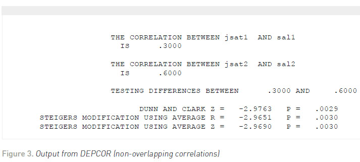
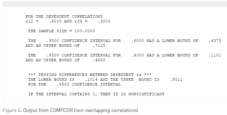
Regardless of the test used, we would conclude that there is a significantly higher correlation between job satisfaction and salary at the end of the year (after the 6% raise was given) than in the beginning of the year. Once again, Zou (2007) developed a confidence interval approach for testing this hypothesis, which purportedly has a nominal (e.g., .95) coverage rate. Using the same correlations, the output from COMPCOR is shown in Figure 4 . The confidence interval limits fall around .1014 and .5011. Because the confidence interval does not fall around zero, then this indicates a statistically significant result (p <.05).

TESTING DEPENDENT PART CORRELATIONAL HYPOTHESES

Finally, Malgady (1987) proposed tests of significance between zero-order and part correlations, part correlations with different predictors and covariates, part correlations with the same predictor and different covariates, and part correlations with different predictors and the same covariate. Examples for applications of these hypotheses with regard to multifaceted personality scales can be found in Hittner (2000).

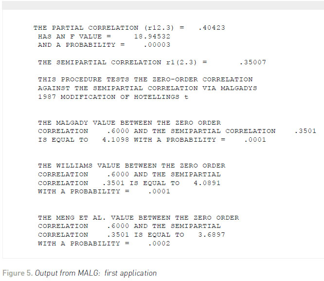
For the first application, suppose that a researcher is interested in examining the difference between the correlation of job satisfaction and salary and job satisfaction and salary removing the effects of supervisory ratings from salary (the part correlation). The program MALG (Hittner, Finger, Mancuso, & Silver, 1995) is user-friendly and interactive querying the researcher for the particular application, sample size, variable labels, and correlations. The output from the first part of the program includes the partial and part correlations along with the Malgady modification and other potential methods.

Suppose that the correlation between job satisfaction and salary is .60, the correlation between job satisfaction and supervisory ratings is .50, and the correlation between salary and supervisory ratings is .70 for 100 elementary school teachers. Figure 5 illustrates the output from the first application. Given the statistical significance of the Malgady value, the conclusion would be that supervisory ratings confounded the relationship between job satisfaction and salary.

Within the literature, Hill, Hall, and Appleton (2010) examined the relationship between self-oriented perfectionism and personal standards with selforiented perfectionism and personal standards removing the effects of conscientiousness achievement striving for self-oriented perfectionism. Moreover, Kalick, Zebrowitz, Langlois, and Johnson (1998) also used this approach in a health context.

The second application examines the differences between two part correlations based on common predictors and covariates. For example, does the correlation between job satisfaction and salary removing the effects of supervisory ratings from salary differ from the correlation between job satisfaction and supervisory ratings removing the effects of salary from supervisory ratings? Using the same correlations and sample size from the previous example, the output from MALG is presented in Figure 6 :

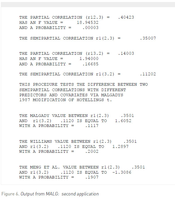
If there was a statistically significant difference between the part correlations, then it would indicate differential predictor-covariate confounding. In this case, there was no predictor-covariate confounding. In the literature, Spinath and Spinath (2005) examined children’s selfperception of their ability predicted from teacher’s rated school achievement and parental perceptions. These predictors were used together and as part correlations.

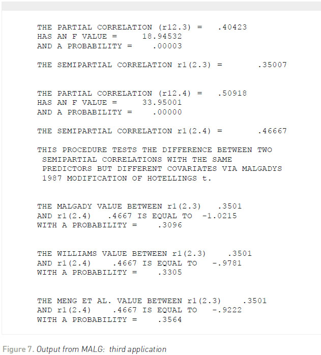
In the third application, the same predictor is used, but there are two different covariates; that is, which of the covariates has a greater confounding effect on the predictor-criterion relationship? For example, suppose the researcher is interested in determining the difference between the correlation of job satisfaction and salary removing the effects of supervisory ratings from salary or removing the effects of experience from salary. Using the same correlations from previous examples, including the correlation between job satisfaction and experience as .40, the correlation between salary and experience as .80, and the correlation between supervisory ratings and experience as .30, then the MALG output for testing this question is shown in Figure 7 . If there was a statistically significant difference between the part correlations, then it would indicate that one covariate (either supervisory ratings or experience) would exhibit the greater confounding effect. Because there was no statistically significant difference in our example, then there is no difference in the confounding effects between supervisory ratings or experience.

From the literature, Sidanius, Kteily, Levin, Pratto, and Obaidi (2016) demonstrated that a perceived clash of cultures and Arab identification were stronger predictors of fundamentalist violence support than American domination.

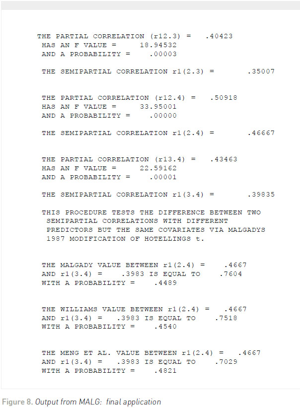
For the final application, the part correlations have different predictors but similar covariates. For example, does the correlation between job satisfaction and salary removing the effects of experience from salary differ from the correlation between job satisfaction and supervisory ratings removing the effects of experience from supervisory ratings? Once again, using the same correlations and sample size, Figure 8 provides the output from MALG. If there was a statistically significant difference between the two part correlations, then the smaller of the two part correlations would indicate which predictor is more susceptible to confounding with regard to experience. In this case, neither supervisory ratings nor salary are more susceptible to confounding with regard to experience.

Although Malgady (1987) proposed these procedures using Hotelling’s t, given the simulation by Hittner et al. (2003), it is equivocal how robust this approach is in terms of Type I error and power. Therefore, the Meng et al. (1992) approach might be a more viable one given that it has a better Type I error rate (albeit slightly conservative) and is more stable (i.e., less of a range of Type I error rate in the simulation) as compared to the other aforementioned procedures.

FINAL COMMENTS

In this article, we have examined a number of different hypothesis testing techniques for dependent correlations which are not readily available using the standard statistical software packages. Although many of these techniques are programmed in R (Diedenhofen & Musch, 2015), it is feasible that many researchers either are unfamiliar with R or are interested in researching their own interests rather than taking the time to learn a new statistical program. Therefore, the programs described in this article run in a Windows PC environment, are user-friendly, and the user needs no programming experience. Each program queries the user to input information from the correlational output of any standard statistical software package. The programs DEPCOR and MALG may be obtained through the website http://www.cofc.edu/~hittnerj/software/software.htm. All programs may be obtained by e-mailing N. Clayton Silver at fdnsilvr@unlv.nevada.edu.

REFERENCES

Boyer, J. E., Palachek, A. D., & Schucany, W. R. (1983). An empirical study of related correlation coefficients. Journal of Educational Statistics, 8(1), 75-86.

Diedenhofen, B. & Musch, J. (2015). cocor: A comprehensive solution for the statistical comparison of correlations. PLoS One, 10(4) doi: http://dx.doi.org/10.1371/journal.pone:0121945

Dunn, O. J., & Clark, V. A. (1969). Correlation coefficients measured on the same individuals. Journal of the American Statistical Association, 64(325), 366-377.

Grygiel, P., Humenny, G., Rebisz, S., Świtaj, P., & Sikorska, J. (2013). Validating the Polish adaptation of the 11-item De Jong Gierveld Loneliness Scale. European Journal of Psychological Assessment, 29(2), 129-139. doi: http://dx.doi. org/10.1027/1015-5759/a000130

Hendrickson, G. F., Stanley, J. C., & Hills, J. R. (1970). Olkin’s new formula for significance of r₁₃ vs r₂₃ compared with Hotelling’s method. American Educational Research Journal, 7(2), 189-195. doi: http://dx.doi.org/10.3102/00028312007002189

Hill, A. P., Hall, H. K., & Appleton, P. R. (2010). A comparative examination of the correlates of self-oriented perfectionism and conscientious achievement striving in male cricket academy players. Psychology of Sport and Exercise, 11(2), 162-168. doi: http://dx.doi.org/10.1016/j.psychsport.2009.11.001

Hittner, J. B. (2000). Novel methods for analyzing multifaceted personality scales: Sense of coherence and depression as an example. The Journal of Psychology, 134(2), 199-209. doi: http://dx.doi.org/10.1080/00223980009600862

Hittner, J. B., May, K., & Silver, N. C. (2003). A Monte Carlo evaluation of tests for comparing dependent correlations. The Journal of General Psychology, 130(2), 149-168. doi: http://dx.doi. org/10.1080/00221300309601282

Hittner, J. B., Finger, M. S., Mancuso, J. P., & Silver, N. C. (1995). A Microsoft FORTRAN 77 program for contrasting part correlations and related statistics. Educational and Psychological Measurement, 55(5), 777-784. doi: http://dx.doi. org/10.1177/0013164495055005010

Hotelling, H. (1940). The selection of variates for use in prediction, with some comments on the general problem of nuisance parameters. Annals of Mathematical Statistics, 11(3), 271-283.

Kalick, S. M., Zebrowitz, L. A., Langlois, J. H., & Johnson, R. M. (1998). Does human facial attractiveness honestly advertise health? Longitudinal data on an evolutionary question. Psychological Science, 9(1), 8-13. doi: http://dx.doi.org/10.1111/1467 9280.00002

Kemtes, K. A., & Allen, D. N. (2008). Presentation modality influences WAIS Digit Span performance in younger and older adults. Journal of Clinical and Experimental Neuropsychology, 30(6), 661-665. doi: http://dx.doi.org/10.1080/13803390701641414

Malgady, R. G. (1987). Contrasting part correlations in regression models. Educational and Psychological Measurement, 47(4), 961-965. doi: http://dx.doi.org/10.1177/0013164487474011

May, K., & Hittner, J. B. (1997). Tests for comparing dependent correlations revisited: A Monte Carlo study. The Journal of Experimental Education, 65(3), 257-269. doi: http://dx.doi.org/ 10.1080/00220973.1997.9943458

Meng, X. L., Rosenthal, R., & Rubin, D. B. (1992). Comparing correlated correlation coefficients. Psychological Bulletin, 111, 172-175. doi: http://dx.doi.org/10.1037/0033-2909.111.1.172

Neill, J. J., & Dunn, O. J. (1975). Equality of dependent correlation coefficients. Biometrics, 31(2), 531-543. Olkin, I. (1967). Correlations revisited. In J. C. Stanley (Ed.), Improving experimental design and statistical analysis (pp. 102-128). Chicago: Rand McNally.

Pearson, K., & Filon, L. G. N. (1898). Mathematical contributions to the theory of evolution. IV. On the probable errors of frequency constants and on the influence of random selection on variation and correlation. Transactions of the Royal Society London (Series A), 191, 229–311. doi: http://dx.doi.org/10.1098/ rsta.1898.0007

Schroeder, P. J. (2014). The effects of age on processing and storage in working memory span tasks and reading comprehension. Experimental Aging Research, 40(3), 308-331. doi: http:// dx.doi.org/10.1080/0361073X.2014.896666

Sidanius, J., Kteily, N., Levin, S., Pratto, F., & Obaidi, M. (2016). Support for asymmetric violence among Arab populations: The clash of cultures, social identity, or counterdominance? Group Processes & Intergroup Relations, 19(3), 343-359. doi: http:// dx.doi.org/10.1177/1368430215577224

Silver, N. C., & Dunlap, W. P. (1987). Averaging correlation coefficients: Should Fisher’s z transformation be used? Journal of Applied Psychology, 72, 146-148.

Silver, N. C., Hittner, J. B., & May, K. (2004). Testing dependent correlations with nonoverlapping variables: A Monte Carlo simulation. The Journal of Experimental Education, 73, 53-69. doi: http://dx.doi.org/10.3200/JEXE.71.1.53-70

Silver, N. C., Hittner, J. B., & May, K. (2006). A FORTRAN 77 program for testing dependent correlations. Applied Psychological Measurement, 30(2), 152-153. doi: http://dx.doi. org/10.1177/0146621605277132

Silver, N. C., Ullman, J. R., & Picker, C. (2015). COMPCOR: A computer program for comparing correlations using confidence intervals. Psychology and Cognitive Sciences, 1, 26-28.

Spinath, B., & Spinath, F. M. (2005). Development of self-perceived ability in elementary school: The role of parents’ perceptions, teacher evaluations, and intelligence. Cognitive Development, 20(2), 190-204. doi: http://dx.doi.org/10.1016/j.cogdev.2005.01.001

Steiger, J. H. (1980). Tests for comparing elements of a correlation matrix. Psychological Bulletin, 87(2), 245-251. doi: http:// dx.doi.org/10.1037/0033-2909.87.2.245

Wilcox, R. R., & Tian, T. (2008). Comparing dependent correlations. The Journal of General Psychology, 135, 105-112.

Wilker, S., Pfeiffer, A., Kolassa, S., Koslowski, D., Elbert, T., & Kolassa, I. T. (2015). How to quantify exposure to traumatic stress? Reliability and predictive validity of measures for cumulative trauma exposure in a post-conflict population. European Journal of Psychotraumatology, 6. doi: http://dx.doi.org/10:3402/ejpt. v6.28306

Williams, E. J. (1959). The comparison of regression variables. Journal of the Royal Statistical Society, Series B, 21(2), 396-399.

Yoo, H. C., Steger, M. F., & Lee, R. M. (2010). Validation of the subtle and blatant racism scale for Asian American college students (SABR-A²). Cultural Diversity and Ethnic Minority Psychology, 16(3), 323-334. doi: http://dx.doi.org/10.1037/a0018674

Zou, G.Y. (2007). Toward using confidence intervals to compare correlations. Psychological Methods, 12(4), 399-413. doi: http://dx.doi.org/10.1037/1082-989X.12.4.399

 

*Email: fdnsilvr@unlv.nevada.edu  **Email: cmerinos@usmp.pe , sikayax@yahoo.com.ar

 

Recibido: 15/09/16

Revisado: 07/10/16

Aceptado: 30/11/16

Publicado: 05/12/16