


 Inglés (pdf)
 Articulo en XML
 Referencias del artículo
 Enviar articulo por email
 Citado por SciELO
  Similares en
SciELO
Similares en
SciELO 
 Permalink
1. INTRODUCTION
Computer vision is the science of extracting information and knowledge from images in order to provide an understanding of the world based on camera observations. Currently, the research on autonomous vehicles has driven many technological advances in computer vision methods and applications. Some of the state-of-the-art computer vision algorithms are 3-D reconstruction from multiple camera views, visual odometry (VO) and visual SLAM (simultaneous localization and mapping or structure from motion), which enable many applications such as autonomous navigation, scene reconstruction, map creation and exploration, etc.
In this work we present a tutorial on the use of computer vision applied to solve actual problems in the automotive industry. More specifically, we present algorithms for the use cameras as measuring devices including edge and ellipse detection, camera calibration, 3-D reconstruction and stereo vision. We motivate these algorithms with three industrial applications: Detection of wheel rims; a system to estimate the calibration angles of vehicles and; the reconstruction of the trajectory of a vehicle using stereo vision.
This tutorial is referenced on a previous work in computer vision [1], but with dedicated attention to the applications in the automotive field including extended theory and results. Therefore, it can be used as a self-contained introduction for engineers and practitioners to motivate further developments that use computer vision in the automotive industry and related fields. The methods were carefully selected according to the challenges presented on each application. For instance, objection detection tasks on Section 2.1 and Section 2.2 are solved using shape detection techniques. Section 2.3 to Section 2.5 introduce the fundamental techniques for the use of cameras as measuring devices allowing metrology applications such as measuring angles and trajectories.
The applications provide computer vision methodologies at an entry level to important problems in Advance Driver Assistance Systems (ADAS), Wheel Alignment and Mobile Robotics. More specifically, the first application discusses how to detect rounded shapes in images, which is important for obstacle avoidance [2], the second application shows an automatic approach for detecting the wheel alignment angles of vehicles using cameras as a low cost alternative to laser-based devices [3] and, finally, the third application shows an application of stereo vision in visual odometry to recover the trajectory of a car-like robot in adverse scenarios where satellite information from the GPS is not accessible [4].
The text is organized as follows: Section 2 presents the theory and foundations of computer vision methods; Section 3 presents three applications of these methods in the automotive industry and robotics; Section 4 outlines the final remarks and conclusions.
2. Computer vision methods
In this section we make a summary of selected computer vision methods and theory required for the applications introduced in the following sections.
2.1 Edge detection
The edges of an image are regions characterized by high changes of pixel intensities [5]. The image edges provide a rich source of information and a simplified representation of a complex image. Edges can be used to detect shapes in object detection tasks such as the lines of buildings or roads, or either to isolate geometrical shapes such as rounded objects (e.g. cells, wheels, balls).
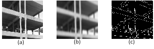
One of the most popular edge detectors was proposed by Canny in [6]. The Canny’s algorithm consists of convolving a grayscale image with a smoothing filter, typically a Gaussian square subimage, to obtain a coarse depiction of the original image. A binary threshold is applied to the smoothed intensities and the regions with the most salient changes are identified as the image edges. Fig. 1a shows the image of a building with pillars showing predominant straight-line edges. The image is convolved with a Gaussian filter and the result of the thresholding process is shown on Fig. 1 with the image edges depicted as white lines.
2.2 Ellipse detection
Shape detection methods are instrumental for identifying the geometrical shapes of objects in images. The detection of shapes has a wide variety of applications such as robot localization [5] object measurement [7], counting [8] and identification [9]. In the automotive industry, detecting wheel shapes may be useful for applications such as measuring wheel dimensions for detecting anomalies or identifying wheeled vehicles for obstacle avoidance on the road such as bicycles, motorcycles and cars.
One of the most popular shape detectors is the so called Hough transform [10], [11]. The Hough transform operates over the edges of an image and is based on a voting principle which consists in parametrizing the shape to be detected (e.g., a line or an ellipse) to produce a mapping of the edge intensities to a space of parameters. An accumulator is incremented on each point coincidence of the curves in the parameter space and the voting is to choose among accumulator cells with the highest count representing the parameters of the detected shape.
The parametrization of an ellipse of coordinates (u,v) is given by
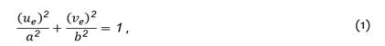


where u 0 and v 0 are the coordinates of the ellipse center, a and b are the lengths of the semi-major and the semi-minor axes, respectively, and Θ is the ellipse rotation angle.
2.3 Camera calibration
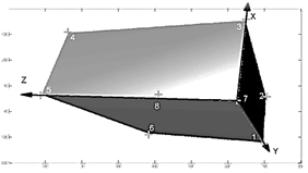
Camera calibration is the process of determining the parameters of a camera required to use it as a measuring device in computer vision and metrology applications. The camera parameters consist of the intrinsics (focal length, principal point, lens distortion) and the extrinsics (rotation and translation with respect to world coordinates). The following camera calibration procedure, based on the work in [12], uses a solid box as calibration pattern as depicted in Fig. 2.
The reference points for calibration are the positions of the eight vertices of the box in world coordinates B k and their pixel mappings p ̂k, with k=1,…,8; they are related by

Calibration consists in estimating the unknowns in ¡Error! No se encuentra el origen de la referencia., which are the depths zk, the matrix of intrinsic, parameters K the rotation R, and translation t. The procedure consists of grouping sets of three different vertices, denoted Bka , Bkb and Bkc , and their corresponding pixel mappings p ̂ka , p ̂kb and p ̂kc

where ⊗ denotes the Kronecker product, I is the identity matrix of size 3, vec(∙) denotes the matrix to vector operator which stacks the columns of matrix KR to yield a vector of size 9, BkI and BkII are defined as


and the matrices P ̂kI and P ̂kII are defined as


and matrix KR is defined as

Equation (5) is extended adding n≥3 different sets of box vertices and their corresponding pixel mappings to form an overdetermined system of equations
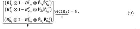
Equation (11) is a system of 3n×9 homogeneous equations with solutions in the right null space of P. However, the matrix P may not have a null space since the pixel positions of the box vertices are only calculated approximately. Hence, the vector x will be estimated as the right-singular vector of P associated to the least non-zero value. The vector x is reshaped into a matrix K R of size 3, which is an estimate of matrix K R,

By exploiting the orthogonal property of the rotation in ¡Error! No se encuentra el origen de la referencia., an estimate of the product of the matrix of intrinsic parameters K and its transpose K T can be derived as
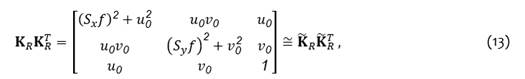
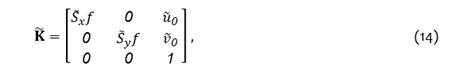
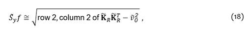
where matrix K R K R T is the normalized version of K R K R T, obtained by imposing its third row, third column element to be 1, as in the same element of KK T. The estimate of the matrix of intrinsic parameters, denoted K ̃, is obtained from the elements of KR K R T, as


A first approximation of the rotation is derived from (10) and the results of (14) and (12), as

To satisfy the orthogonal property of rotations, the final rotation estimate, denoted R, is obtained from the singular value decomposition (SVD) of matrix K -1 K R

where U and V are matrices of the left and right singular vectors of K -1 K R, respectively.
The estimate of the vector of depth reprojections, denoted λ, and the translation vector, denoted t, are obtained simultaneously by extending ¡Error! No se encuentra el origen de la referencia. to n≥2 different pairs of vertices and their pixel mappings, and solving for
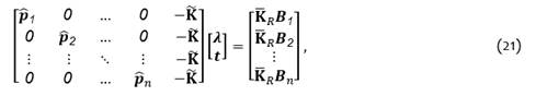
where λ is defined as

2.4 3-D reconstruction
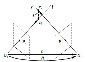
Fig. 3 depicts the 3-D reconstruction of a point in the space P ⋆ by triangulation. Triangulation consists of finding the closest point between the rays l=(Ol,pl ) and r=(Or,pr ) from the origins of left and right cameras to the point P. An optimal solution to the 3-D reconstruction problem is obtained by minimizing the geometric error in spatial position and solving for depths zl and zr


where e is the error vector in spatial position of crossing rays, p l and p r are normalized pixel coordinates (focal length f=1m) and (R,t) are the extrinsic parameters denoting the transformation between camera views.
2.5 Stereo vision
Two camera views are related by epipolar geometry or the geometry of stereo vision. Figure 4 illustrates the epipolar relations. The line connecting the camera projection centers is called baseline. The baseline intersects the image planes πl and πr at special points called epipoles el and er. A point in the 3-D space P is described by the vectors Pl=[xl yl zl ) ]T and Pr=[xr yr zr ) ]T and the camera projections pl=[xl yl fl ) ]T and pr=[xr yr fr ) ]T, where fl and fr are the focal lengths. The point P and the projection centers Ol and Or describe a plane πP called epipolar plane (in gray color). The lines connecting the epipoles to the camera projection centers are called epipolar lines, denoted ul and ur. The stereo configuration also imposes the epipolar constraint which restricts the match of a point in an image to the epipolar line on the opposite image.
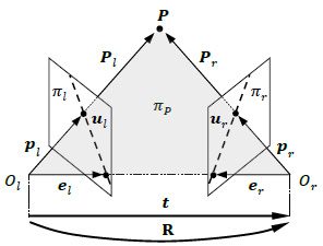
The translation vector t and rotation matrix R are the extrinsic parameters that relate the reference frames of the left and right cameras. Then, the points Pl and Pr are related by the rigid body transformation

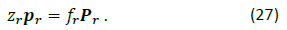
The point P is related to its perspective projection p using the standard pinhole camera model

The essential matrix E of camera coordinates establishes an epipolar constraint between the left and right projections
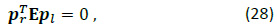
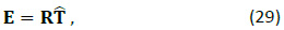
where T ̂ is the skew-symmetric matrix expressing the cross product with the translation vector t×(∙). The points pl and pr are the pixel mappings in homogenous coordinates corresponding to p l and pr
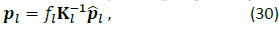
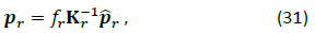
where K l and K r are the calibration matrices of the left and right cameras, respectively.
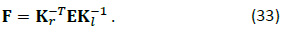
The fundamental matrix F of image coordinates establishes the epipolar constraint between the left and right projections as
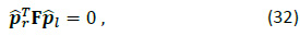
Matrices E and F can be estimated using the eight-point algorithm [9]
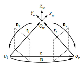
Fig. 5. The extrinsic parameters of a stereo system.
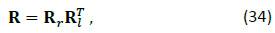
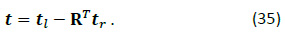
shows the geometric relations between the cameras and the world. Rotations Rl and Rr and translations tl and tr describe the origin of world coordinates Ow in terms of the reference frames of the left and right cameras, respectively. The extrinsic parameters of the stereo system R and t are calculated with respect to the reference frame of the left camera, such as
3. Automotive applications
In this section we present three applications of computer vision methods in the automotive industry and robotics. In order to highlight the potential of the methods, we make use of simulations using Blender, which is an open-source platform used for generating virtual scenarios as ground truth data for evaluation [13], [ 14;1]. In Section 3.1, real images of a wheel were used. In Section 3.2, we used the 3-D model of a vehicle and an array of eight cameras grouped in pairs, as in Fig. 8. In Section 3.3, we used a 3-D indoors environment comprised of texturized furniture, chairs, floor, ceiling, windows, natural and artificial illumination to enable the detection of visual keypoints. A 3-D model of an automotive vehicle with a mounted pair of stereoscopic cameras is also introduced in the environment. The car-like robot simulates an autonomous vehicle following a predefined trajectory inside a virtual environment, capturing stereo images. The ground truth path contains straight and diagonal trajectories with rotations at different angles.
3.1 Detection of wheel rim
In this application we describe a method for detecting rims in automotive wheel images using the Hough transform. Rim detection may be useful to identify wheeled vehicles in tracking applications [2]. Fig. 6a depicts a wheel image originally affected by poor illumination and lens distortion which are corrected using the histogram equalization and correction of lens distortion. Fig. 6b shows the resulting image including both corrections.
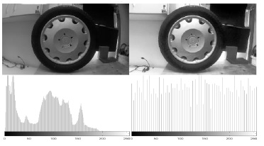
The ellipse containing the wheel rim is detected using the Hough transform applied to elliptical shapes [15], [16]. The procedure starts by converting the RBG image to grayscale intensities

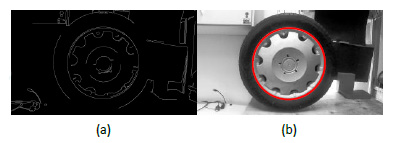
The Canny algorithm is computed over the grayscale image in order to detect the edges of the wheel. The rim ellipse is searched over the image edges using the ellipse parametrization given in (1-2). Fig. 7 illustrates the detection results. Fig. 7b represents the detected wheel rim ellipse in red thick line.
3.2 Toe and camber calibration angles
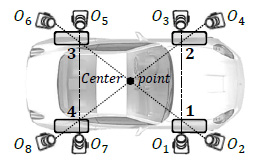
In this application we describe a system to recover the calibration angles of a vehicle. The system can be used as an automatic system to measure the wheel geometry and also to determine the toe and camber calibration angles. Fig. 8 depicts the measuring system consisting of four stereo camera subsystems associated to wheels 1, 2, 3 and 4. The stereo subsystems are attached to a support of fixed baseline to have the center of the wheels and the optical axes of the cameras aligned at approximately the same height. The cameras are oriented towards the wheels and operate in precision and reference positions. Precision cameras 1, 3, 5 and 7 are perpendicular to the wheels to capture the largest possible images of the rims. Reference cameras 2, 4, 6 and 8 are oriented towards the geometric center of the system to capture images of the rims.
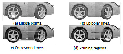
Rim ellipses are detected using the procedure described in previous section. Fig. 9a shows the wheel images of cameras 7 and 8 and the identified rim ellipses (in dotted lines). The rim points on the left image are associated to epipolar lines on the right image due to the epipolar constraint. Epipolar lines intersect the rim ellipse at two points, as shown in Fig. 9b. The epipolar lines of the upper and lower sections of the rim at 10% of the rim diameter are filtered out, as shown in Fig. 9d.
a illustrates the result of the 3-D wheel rim reconstruction. The 3-D wheel rim is reconstructed by triangulation of corresponding 2-D rim points using ¡Error! No se encuentra el origen de la referencia.. The wheel axis system is an auxiliary reference frame defined as the orthogonal 3-D basis resulting from the Principal Component Analysis (PCA) of the 3-D wheel rim, as illustrated in Fig. 10b. The vectors u and v are located on the wheel rim plane and the vector 𝒘 is collinear with the wheel spin axis. The local PCA coordinates are converted to global coordinates in the world reference frame using the extrinsic parameters of the global calibration process of the corresponding stereo subsystem.
The camber and toe alignment angles of the front wheels are measured in a 3-D global system called the car reference frame defined by axis 𝑥 ′ in the direction of the line that connects the centers of wheels 3 and 4, axis 𝑦 ′ defined in the direction of the line that connects the centers of wheels 3 and 2 and axis 𝑧 ′ given by the cross product of 𝑥 ′ and 𝑦 ′ . The triad 𝑥 ′ , 𝑦 ′ and 𝑧 ′ is normalized to yield the unit vectors 𝑥 , 𝑦 and 𝑧 denoting the car reference frame.

Fig. 11a depicts the location of the wheel spin axes in the car reference frame. Vectors w1, w2, w3 and w4 are collinear with the wheel spin axes and perpendicular to wheels 1, 2, 3 and 4, respectively. Vectors w3 and w4 are approximately collinear with the x-axis. Vectors w1 and w2 are perpendicular to the misaligned wheels 1 and 2, respectively.
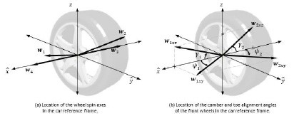
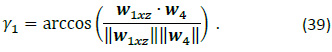
Fig. 11b depicts the location of the wheel alignment angles in the car reference frame. Vector w1xz is the projection of w1 onto the xz plane. The camber angle of wheel 1, denoted γ_1, is the angle from w1xz to the x ̂-axis and is calculated as
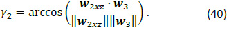
Vector w2xz is the projection of w2 onto the x z plane. The camber angle of wheel 2, denoted γ_2, is the angle from w2xz to the -x-axis and is calculated as
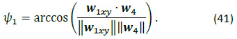
Vector w1xy is the projection of w_1 onto the xy plane. The toe angle of wheel 1, denoted ψ1, is the angle from w1xy to the x -axis and is calculated as
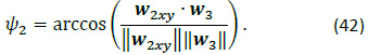
Vector w2xy is the projection of w2 onto the xy plane. The toe angle of wheel 2, denoted ψ2, is the angle from w2xy to the -x-axis and is calculated as
3.3 Visual odometry
Visual odometry (VO) is a technique to estimate the ego-motion of a vehicle using imaging sensors. VO has gained recent attention as a technique to achieve autonomous navigation in mobile robotics. In the following application the path of robot moving in an unstructured environment is recovered using a stereo camera system in a simulated scenario [17].
The system setup consists of two cameras of 720×480 resolution and fixed baseline mounted on a mobile robotic platform. The extrinsic parameters of the stereo system are rotation matrix R and translation vector t, as in Fig. 4. Calibration is performed using the algorithm introduced in previous section to determine the intrinsic and extrinsic camera parameters. Local robot motion is estimated in the robot reference frame located at the projection center of the left camera. The world reference frame is arbitrarily located at the origin of the left camera at the initial position of the robot.
The image matching is based on a practical implementation of the SIFT algorithm [18]. Four stereo images are captured at consecutive robot steps i-1 and i, where i ∈N. The images are analyzed as in the sequence of Fig. 12. The image planes πl and πr represent the left and right camera images, respectively. The main assumption is that consecutive images preserve keypoint correspondences whenever the robot undergoes a small displacement. The set of common keypoints between the four images is the input data for VO estimation.
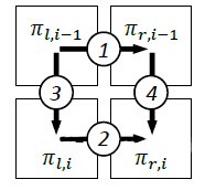
Fig. 13 illustrates the keypoint correspondences at two successive robot steps. Local robot motion is represented by rotation matrix Ri and translation vector ti. Local robot motion is recovered from the 3-D reprojections of the keypoints on the left camera, denoted Pk and Qk, at robot steps i-1 and i, respectively, where k is the keypoint index. The 3-D reprojections are calculated by triangulation, as in ¡Error! No se encuentra el origen de la referencia.
The results are arranged in matrices of homogeneous coordinates P and Q of size 4×k, according to
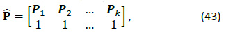
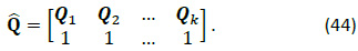
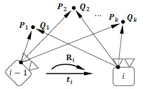
Local robot motion is estimated from the submatrices of the block matrix M (transformation matrix) that relates matrices P and Q, such as
where Ri is the 3×3 rotation matrix and ti is the 3×1 translation vector, and 0T is a zero matrix of size 3×1.
Visual odometry is calculated by the composition of successive rotations and translations. The robot pose, denoted Bi, can be defined recursively as
or as in the explicit version
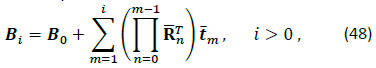
where B0 is the initial robot pose, R0=I3, and I3 is the identity matrix of size 3.
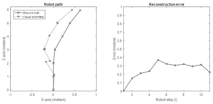
The system is simulated in the 3-D graphics software Blender. In this application, a 3-D virtual indoors environment is used. The environment is comprised of textured office furniture, floor, ceiling, windows, and artificial illumination. A mobile robot is simulated by a stereo camera system of fixed baseline. The robot moves inside the virtual environment on a predefined trajectory, capturing images from both cameras as it traverses small increments of the distance along the path. Fig. 14 depicts the reconstruction of a robot trajectory with i=11 steps. The ground truth trajectory contains straight and diagonal paths and rotations at different angles. The deviation error of the reconstructed path is measured in units of length as
where Bi and Bi are the estimated and the actual robot poses at step i, respectively. VO yields a Gaussian error distribution of mean μ=0.2488m and standard deviation σ=0.1035m. The VO algorithm is plausible of being implemented in real-time scenarios [19]. The results may be improved in combination with state-of-the-art techniques in visual navigation for autonomous vehicles [4], [20] .
Conclusions
In this paper we reviewed computer vision methods applied to automotive applications. The methods presented included edge and ellipse detection, camera calibration, 3-D reconstruction and stereo vision which in group constituted the foundations for the use of cameras as measuring devices.
The automotive applications were the detection of wheel rim, the estimation of toe and camber calibration angles and a visual odometry system using a pair of cameras. The results demonstrated the potential of computer vision methods in solving actual problems of industrial relevance in automotive industry.

