


 Inglês (pdf)
 Artigo em XML
 Referências do artigo
 Enviar este artigo por email
 Citado por SciELO
  Similares em
SciELO
Similares em
SciELO 
 Permalink
1. INTRODUCTION
The fluid-structure interaction is the physical phenomenon that modifies the dynamic response of a structure in contact with a fluid. The slenderness and flexibility of arch dams increase the interaction with the reservoir, this modifies the dynamic characteristics of the dam and; therefore, the dynamic response to earthquakes1.
Westergaard, in the early 1930s, proposed a pseudo-static formulation to estimate the hydrodynamic pressures in a concrete dam based on certain simplifications2, further this formulation was known as Westergaard's added mass. Subsequently, this formulation was generalized to include the flexibility and double curvature of arch dams3, but still with certain limitations. More recent formulations, based on numerical methods, were developed with the advance of computers4 being the most common the Eulerian5 and Lagrangian6 formulations. These formulations try to deal with the simplifications introduced by Westergaard; however, they are not exempt of practical difficulties.
The importance to mitigate the risk of arch dams’ failure makes it essential to include criteria not considered in the typical buildings analysis. For this reason, this study compares the dynamic response of a hypothetical arch dam located on the Marañón River considering the fluid-structure interaction under the generalized Westergaard’s added mass, Eulerian and Lagrangian formulations, as well as the dynamic response of the empty-reservoir condition. The finite element method, in COMSOL Multiphysics software, is carried out to perform time-history analyses under earthquakes of different seismogenic source: Moquegua (2001, inter-plate), Tarapacá (2005, intra-plate) and Pisco (2007, inter-plate) assuming linear elastic behavior of the dam and foundation domains and a massless foundation approach.
2. BACKGROUND
In the fluid-structure interaction, each physical domain is described by its own differential equations of motion; however, since it is a coupled phenomenon, it is not possible to determine the solution of one domain independently of the other. Therefore, boundary conditions on the common surface, called fluid-structure interface, are required to obtain the coupled solution7.
The direction, intensity, and frequency content as well as the vertical component of the earthquake and the reservoir boundary conditions are the most relevant factors in the estimation of the hydrodynamic pressure, while the extent of the reservoir is irrelevant for extensions greater than three times the height of the dam1.
2.1 WESTERGAARD’S ADDED MASS FORMULATION
Westergaard, with certain assumptions, estimated that hydrodynamic pressures are approximate to the inertial effects produced by a prismatic body of water firmly added to the upstream face of the dam and forced to oscillate frictionlessly along with the dam, while the rest of the reservoir remains stationary2. These assumptions were: two-dimensional dam of infinite stiffness and vertical upstream face; reservoir of infinite extension in the upstream direction, perfectly incompressible fluid, and small displacements to ignore the effects of surface waves; and ground excitation limited to harmonic oscillation in the upstream-downstream direction with periods greater than 1 second.
Subsequently, this formulation was generalized to include flexibility and double curvature of arch dams, i.e., the direction and magnitude of the hydrodynamic forces vary at each point of the dam3. Also, since the added masses increase the mass of the system without modifying its stiffness, the vibration frequencies of the coupled system are lower than the frequencies of the dam alone, which is expected to occur in the fluid-structure interaction phenomenon. However, this generalization is only an extrapolation of the classical Westergaard formulation; therefore, it still ignores the fluid compressibility and the effects of energy dissipation by waves transmission from the reservoir to the dam and the ground, as well as surface waves dissipation8.
The Generalized Westergaard formulation assumes, like the classical formulation, that the pressure at any point i on the upstream face of the dam is equivalent to consider the inertial effects of a prismatic body of water oscillating with the dam9 as determined by (1) and shown in Fig. 1:
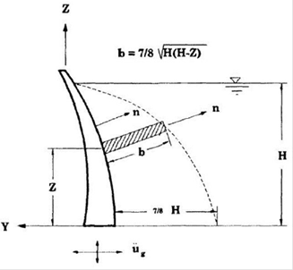
Under the finite element method interpretation, nT üi is the normal component of the acceleration at node i, ρw the water density, H the depth of the reservoir, and Zi the distance from node i to the reservoir bottom. Also, b(Zi) represents the thickness of the prismatic body of water, of unit length in the X direction, at elevation Zi.
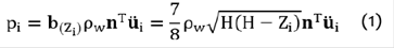
The vector of equivalent inertial forces at node i (Fi) is obtained by multiplying the pressure and the tributary area (nAi) of the node i.

Where mai is the matrix of added mass to node i. Fi is assembled in a similar way to the stiffness matrix; therefore, the matrix of inertial forces (Fa) applied to the dam is:
M a is the matrix of mass to be added in the dam and ü the acceleration vector of the coupled system.

M, C, K are the mass, damping and stiffness matrices for the coupled system, respectively; and ú, u are the velocity and displacement vectors for the coupled system, respectively.
2.2 EULERIAN FORMULATION
2.2.1 Equation of Motion
The equation of motion of the dam-foundation domain (Ωs) is described in terms of displacement, while the fluid domain (Ωf) ones in terms of pressure10. Therefore, compatibility and equilibrium at the interface of both systems is ensured by interface equations. COMSOL Multiphysics considers the pressure as degree of freedom defining the fluid domain as an acoustic domain11.
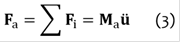
The equation of motion for the fluid domain or Helmholtz equation (5) is obtained by combining the Navier-Stokes and continuity equations under the Eulerian approach, previously simplified by the following hypothesis: low fluid compressibility, low velocities, and ignore viscous effects as well as body forces7.
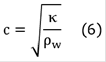
Where ∇ is the gradient operator, p the hydrodynamic pressure and ṗ its second derivative with respect to time, and c the speed of wave sound in water defined in terms of the modulus of compressibility (κ) and the water density as10:
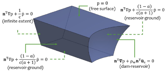
2.2.2 Boundary Conditions
The dam-reservoir interface (ΓI) represents the coupled motion of the dam and the fluid; therefore, the normal displacements at this interface must be compatible in both domains7:
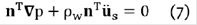
Where nTüs is the normal component of the acceleration in the structure domain.
The reservoir-ground interface (ΓD) represents the phenomenon of energy dissipation by incidence and reflection of pressure waves on the ground10:
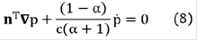
Where ṗ is the first derivative with respect to time of the pressure and α the reflection coefficient defined as the ratio between the amplitude of incident and reflected wave. Typically, it can be considered equal to 0.3 for the sediments deposited on the bottom of the river and equal to 0.7 for the rocks on the lateral slopes.
The free surface (ΓL) represents the phenomenon of energy dissipation by surface waves. Nevertheless, if the energy dissipation by surface waves is ignored, it can be considered that the hydrodynamic pressure is equal to zero at this surface7. This assumption is a valid approximation since the surface waves energy is much smaller than the energy generated by the hydrodynamic pressure.

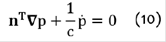
The infinite extension of the reservoir (ΓT) represents the outcoming waves in the normal direction (no incoming waves)7, which is known as the equation of Sommerfield. Fig. 2 shows the boundary conditions.
2.2.3 Discrete Finite Element Formulation
The discrete form of the equation of motion of dam-foundation domain is obtained by the Galerkin’s method and replacing the boundary condition corresponding to the dam-reservoir interface10.

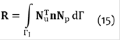
Where Ms, Cs, and Ks are the mass, damping and stiffness matrices respectively for the dam-foundation domain; R the interaction matrix, and Fs ext the vector containing the external forces applied to the system. Moreover, üs, ůs, and ûs are the nodal acceleration, velocity, and displacement vector respectively for the dam-foundation domain and ṗ the nodal pressure vector for the fluid domain.
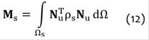
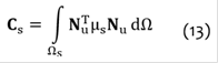


Nu and Np are the shape-functions for the displacement and pressure respectively, ρs the dam-foundation density, μs the dam-foundation viscous damping per unit volume, L the matrix relating strain and displacements, B the matrix relating strain and stress, and bs the body force in the dam-foundation domain.
The discrete form of the equation of motion for the fluid domain is also obtained by Galerkin's method and replacing the boundary conditions10.
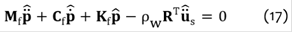
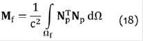
Where Mf, Cf and Kf are the pseudo-mass, pseudo-damping, and pseudo-stiffness matrices respectively for the fluid domain, ¨p and ṗ are first and second derivative with respect to time of the nodal pressure vector respectively.


RT allows to transform the hydrodynamic pressures into forces applied on the structure, as well as the accelerations of the structure into hydrodynamic pressures.
These equations can be rewritten in their coupled form as:

2.3 LAGRANGIAN FORMULATION
2.3.1 Equation of Motion
The equations of motion of the dam-foundation domain as well as the fluid domain are described in terms of displacement12. Moreover, the fluid is assumed to be an elastic and almost incompressible linear material (Poisson’s coefficient close to 0.5) without viscosity and irrotational13.
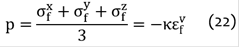
The hydrodynamic pressure at any point is approximated as the mean stress at that point which is defined, for an isotropic material, as the product of the volumetric strain  and the modulus of compressibility7.
2.3.2 Boundary Conditions
The boundary conditions are like those determined in the Eulerian formulation but expressed in terms of displacements. Fig. 3 shows these boundary conditions.
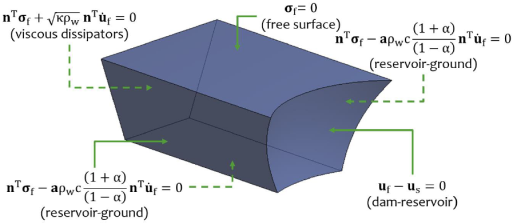
The dam-reservoir interface (ri) given by:
The reservoir-ground interface (ΓD) could typically be represented assuming compatibility of displacements between the ground and the reservoir; however, this would ignore the energy dissipation by incidence of waves in the ground. A better alternative is to use viscous dissipators connecting the ground and the reservoir, whose dissipation coefficient for compressional waves is estimated by equivalence between acoustic and mechanical impedance. Since this equivalence is only an approximation, a correlation factor denoted as a is required. In this study a = 0.5 is considered as values between 0.5 and 0.75 seem to be adequate14.

Where σf is the tensor stress and úf the vector velocity in the fluid domain.
The free surface (ΓL), if it is not considered any constraint on displacements, strains will occur on the surface, which can be interpreted as waves motion.
The infinite extension of the reservoir (ΓT), Lysmer-Kuhlemeyer viscous dissipators15 are placed in the direction normal to the surface to dissipate the compressional waves outcoming and reduce the amplitude of the reflected waves on this boundary.
2.3.3 Discrete Finite Element Formulation
The discrete form of the equation of motion for the dam-foundation domain is like that obtained for the Eulerian formulation except that:
Where ts are the Neumann boundary condition in dam-foundation domain.
A mixed formulation is required to discretize the equation of motion for the fluid domain. The mixed formulation allows expressing the equation in terms of displacement and pressure as independent variables, since, if the equation of motion for the fluid domain is discretized from an irreducible formulation, based on displacements as the only degree of freedom, numerical problems related to volumetric strains may be incurred. These numerical errors occur when considering a high compressibility modulus that fictitiously amplifies the volumetric strains, which in turn generate a fictitious mean stress7. COMSOL Multiphysics considers this mixed formulation selecting the option of Nearly Incompressible Material11.
The discrete form of the equation of motion for the fluid domain is expressed by:
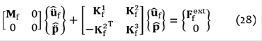
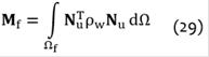
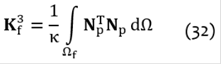
Where the matrices Mf, Ki f , and Ff ext are defined by:
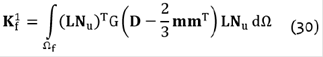

Where G is the shear modulus,  and m=[1,1,1,0,0,0]T
These equations can be rewritten in their coupled form as:
3. METHODOLOGY
The dynamic analyses, in the time domain, are carried out with a direct integration method and the generalized alpha algorithm16, which allows to control the numerical dissipation at high frequencies without introducing considerable dissipation at low frequencies.
Linear and elastic behavior is considered for dam-foundation domain as well as for the fluid domain in the Lagrangian formulation.
3.1 GEOMETRY
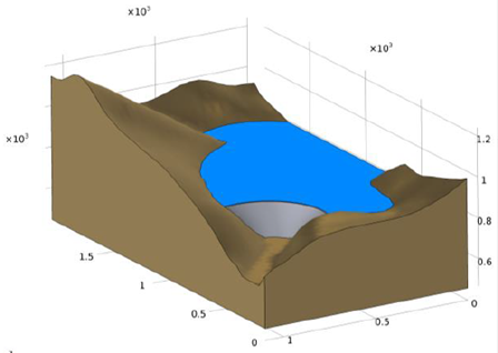
The geometry of the dam follows the recommendations of USACE17: 175m height, 7.8m width at crest and 33.5m width at base. Moreover, foundation and reservoir extension follow the recommendations of Chopra and Fok18 as well as the conclusions provided by Sevim et al.19: 1900m along the X-axis, 1100m along the Y-axis, and 175m below the dam base level for the foundation, and 555m extension in the upstream direction for the reservoir. Fig. 4 shows the dimensions of the finite element model.
3.2 FINITE ELEMENT MODEL
10-node tetrahedral elements of the Lagrangian family with quadratic shape-functions are used. The Westergaard formulation does not require a fluid domain as the water is represented by added masses per unit area on the upstream face of the dam. On the other hand, the fluid domain is represented as a physical domain in both Eulerian and Lagrangian formulations.
Fig.5 shows the quality of the mesh determined by an absolute scale from 0 to 1 (from low to high quality)11. Dam mesh elements are of 15m maximum size and 0.75 average quality, reservoir mesh elements range from 50 to 60m and have 0.67 average quality, and foundation mesh elements range from 50m to 200m and have 0.5 average quality.
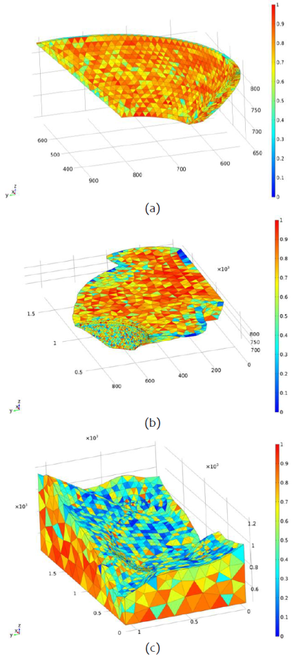
The mesh sizes used to analyze the model consider the User’s guide recommendations of COMSOL Multiphysics for wave propagation problems20. When elements of the Lagrangian family with quadratic shape functions are used, these recommendations establish that: First, it is necessary to define a maximum element size equal to one-fifth of the minimum wavelength to be represented, and then verify if the number of degrees of freedom obtained is at least 1728 times the volume of the model measured in wavelength units.
3.3 MATERIALS
The elastic properties of the concrete dam and the foundation are listed in TABLE I. It is considered 5% Rayleigh damping associated with the first (2.35Hz) and sixth (5.59Hz) vibration modes of the dam-foundation system.
TABLE I Elastic properties of concrete and foundation
| Material | Young’s module (MPa) | Poisson | Density (kg/m3) |
|---|---|---|---|
| Concrete | 38000 | 0.25 | 2300 |
| Foundation (Rock) | 65000 | 0.25 | Massless |
The elastic (Lagrangian formulation) and acoustic properties (Eulerian formulation) of the reservoir (water) are listed in TABLE II.
3.4 DYNAMIC ANALYSIS
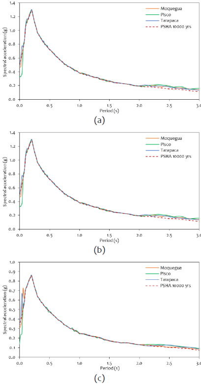
The dynamic time-history analyses are performed for synthetic earthquakes determined for the coast of Peru21, which, following the guidelines of international standards, are previously matched to the uniform hazard spectrum with a return period of 10000 years for the Marañón zone as shown in Fig. 6. Gravity loads are ignored to focus on the dynamic response.
Massless foundation approach is valid to represent the foundation since spatial variations of acceleration along the dam-foundation interface are insignificant in rigid rocks. This approach ignores the effects of waves propagation, but considers the effects of flexibility22.
4. RESULTS
In the following figures, as a convention, it is considered that the positive displacements and accelerations correspond to movements in the upstream direction.
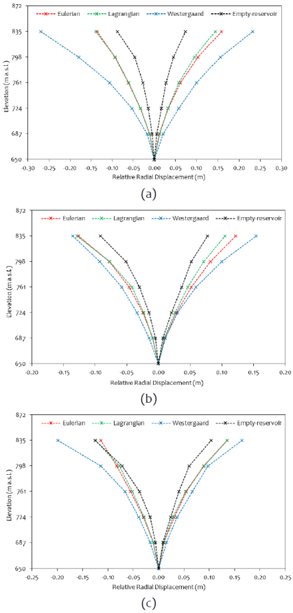
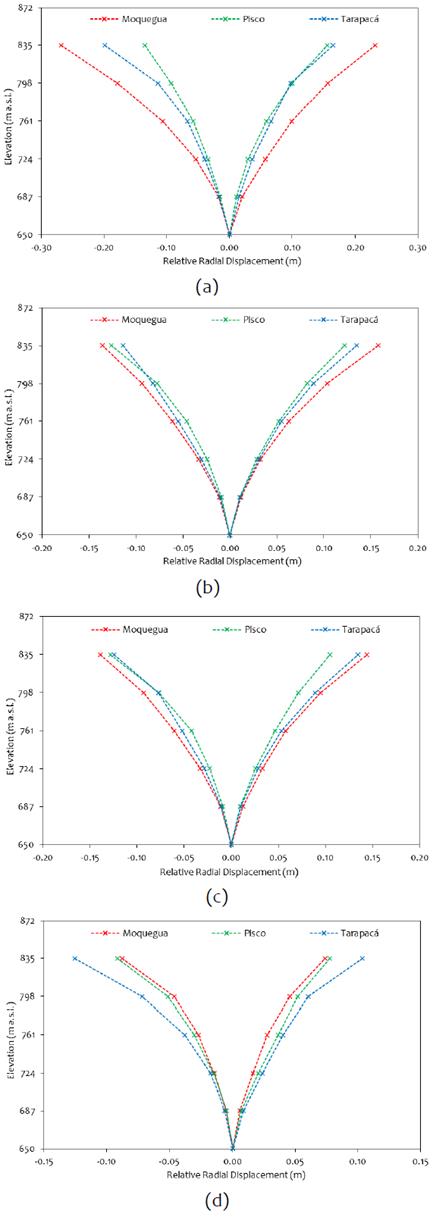
Fig. 7 shows the maximum relative radial displacements in the central section. Westergaard’s formulation produces higher radial displacement than Eulerian and Lagrangian formulations, which produce similar results. Likewise, the empty-reservoir condition produces considerably lower results than the full-reservoir condition, except for the Tarapacá earthquake, which is mainly associated to the frequency content of that earthquake.
Harmonic analyses are carried out in both horizontal directions to illustrate the dependency of the response with the frequency. Fig. 8 shows that empty-reservoir condition produces higher response than Eulerian formulation for some excitation frequencies.
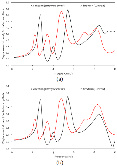
Fig. 9 and 10 show the time-history of the radial relative displacements and the radial absolute accelerations at the crest, respectively. Eulerian and Lagrangian formulations follow the same response pattern, while Westergaard’s formulation and the empty-reservoir condition follow different patterns between them and regarding to the other responses.

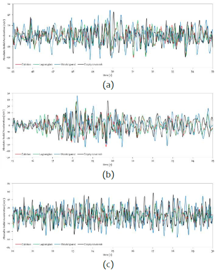
Fig. 11 and 12 show the time-history of hydrodynamic pressures at the bottom of the reservoir (elevation 660 m a.s.l.) and at the mean height of the reservoir (762 m a.s.l.), respectively. Eulerian and Lagrangian formulations follow the same response pattern, from the engineering point of view, while the response for the Westergaard formulation follows a different pattern. Also, hydrodynamic pressure is higher at the mean height than at the bottom of the reservoir as hydrodynamic pressure depends on the acceleration of the dam at each point of the fluid-structure interface in contrast to the hydrostatic pressure that depends only on the depth from the free surface.
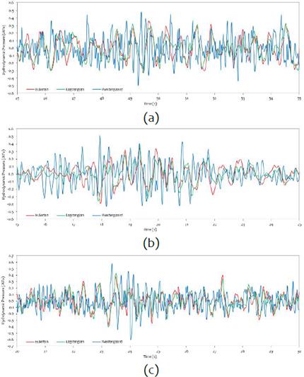
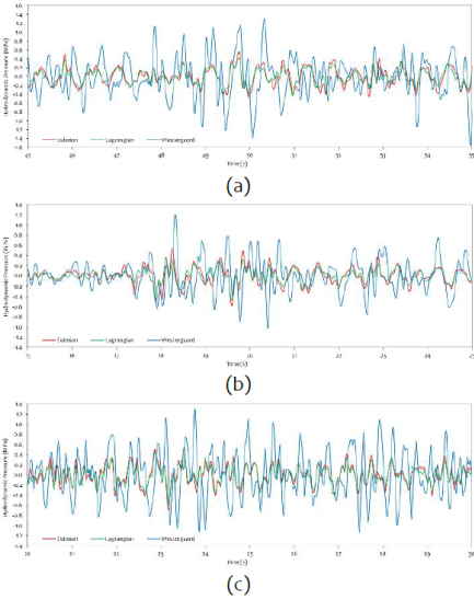
Fig. 12 Hydrodynamic pressure at mean height of the reservoir (a) Moquegua, (b) Pisco, and (c) Tarapacá
Fig. 14 to 15 show the maximum hydrodynamic pressures. Pressure distribution, maximum values as well as the time when they occur are very similar between the Eulerian and Lagrangian formulations.
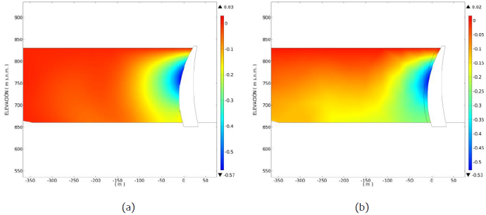
Fig. 14 Maximum hydrodynamic pressure (MPa) Pisco earthquake (a) Eulerian t=19.59 s and (b) Lagrangian t=19.58 s
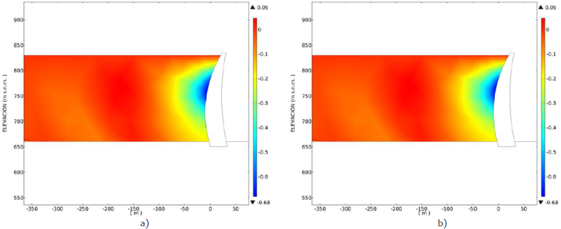
Fig. 15 Maximum hydrodynamic pressure (MPa) Tarapacá earthquake (a) Eulerian t=23.16 s and (b) Lagrangian t=23.17 s
Fig. 16 shows the maximum relative radial displacements in the central section. Eulerian and Lagrangian formulations do not show an important variation between the earthquakes. Nevertheless, Westergaard’s formulation and the empty-reservoir condition do show higher displacement for Moquegua and Tarapacá earthquakes, respectively.
CONCLUSIONS
Westergaard’s formulation produces conservative results compared to the other formulations analyzed. Likewise, Eulerian and Lagrangian formulations will produce similar results, from an engineering point of view, if the appropriate parameters are considered for the variables that define the behavior of the model, such as the elastic constants (Poisson's coefficient and compressibility modulus) and boundary conditions, mainly for energy dissipation at the reservoir-ground interface.
The fluid-structure interaction generally increases the dynamic response of an arch dam with respect to the empty-reservoir condition; however, this will depend on the characteristics of the earthquake considered. As a particular case, in the Moquegua and Pisco earthquakes (inter-plate) a notorious increase of the dynamic response due to the fluid-structure interaction is observed, while in the Tarapacá earthquake (intra-plate) this increase is smaller, even obtaining higher relative radial displacements for the empty-reservoir condition at the elevation near the dam crest respect to Eulerian formulation.
Lagrangian formulation has the advantage that it can be evaluated in many commercial computer programs.

